from sklearn.datasets import load_iris
import matplotlib.pyplot as plt
import pandas as pd

# Load toy dataset
iris = load_iris()
 # Create dataframe using feature names
df = pd.DataFrame(iris.data, columns=iris.feature_names)Notebook Iris Dataset
Before we dive in, here’s a quick summary: the dataset contains 150 samples of iris flowers, each characterized by four features: Sepal Length, Sepal Width, Petal Length, and Petal Width, all measured in centimeters. These samples are grouped into three species: Setosa, Versicolor, and Virginica. If you’re not familiar with the dataset, you can learn more about it here.
1 Loading the dataset
Let’s start by importing the iris dataset and manipulating the dataframe so that the column names match the feature names.
2 Exploring the dataset
Let´s start by exploring the species by plotting the sepal length vs. width in a scatter plot
import matplotlib.pyplot as plt

_, ax = plt.subplots()
scatter = ax.scatter(iris.data[:, 0], iris.data[:, 1], c=iris.target)
ax.set(xlabel=iris.feature_names[0], ylabel=iris.feature_names[1])
_ = ax.legend(
    scatter.legend_elements()[0], iris.target_names, loc="lower right", title="Classes"
)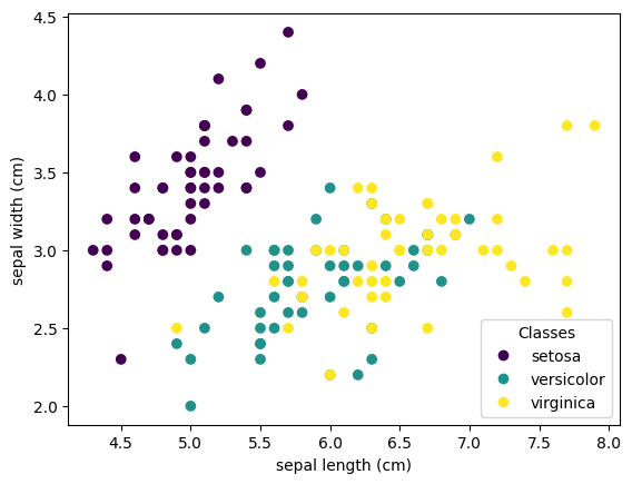
You can already see a pattern regarding the Setosa type, which is easily identifiable based on its short and wide sepal. Only considering these 2 dimensions, sepal width and length, there’s still overlap between the Versicolor and Virginica types.
3 Transforming the dataset
We will now perform feature engineering and create a new feature called petal area (petal length * petal width), and will do the same for the sepal.
df['sepal_area'] = df['sepal length (cm)'] * df['sepal width (cm)']
df['petal_area'] = df['petal length (cm)'] * df['petal width (cm)']
Finally, let’s new information by binning the sepal length into 3 categories (short, medium and long)
df['sepal_length_bin'] = pd.cut(df['sepal length (cm)'], bins=3, labels=["short", "medium", "long"])
df| sepal length (cm) | sepal width (cm) | petal length (cm) | petal width (cm) | sepal_area | petal_area | sepal_length_bin | |
|---|---|---|---|---|---|---|---|
| 0 | 5.1 | 3.5 | 1.4 | 0.2 | 17.85 | 0.28 | short |
| 1 | 4.9 | 3.0 | 1.4 | 0.2 | 14.70 | 0.28 | short |
| 2 | 4.7 | 3.2 | 1.3 | 0.2 | 15.04 | 0.26 | short |
| 3 | 4.6 | 3.1 | 1.5 | 0.2 | 14.26 | 0.30 | short |
| 4 | 5.0 | 3.6 | 1.4 | 0.2 | 18.00 | 0.28 | short |
| ... | ... | ... | ... | ... | ... | ... | ... |
| 145 | 6.7 | 3.0 | 5.2 | 2.3 | 20.10 | 11.96 | medium |
| 146 | 6.3 | 2.5 | 5.0 | 1.9 | 15.75 | 9.50 | medium |
| 147 | 6.5 | 3.0 | 5.2 | 2.0 | 19.50 | 10.40 | medium |
| 148 | 6.2 | 3.4 | 5.4 | 2.3 | 21.08 | 12.42 | medium |
| 149 | 5.9 | 3.0 | 5.1 | 1.8 | 17.70 | 9.18 | medium |
150 rows × 7 columns
4 Computing summary statistics
Now, we can extract summary statistics of the species “setosa” and compare it to another species
# Map targets to species names and add them to a new column
df['species'] = iris.target_names[iris.target]
# Display first few rows
df.head() | sepal length (cm) | sepal width (cm) | petal length (cm) | petal width (cm) | sepal_area | petal_area | sepal_length_bin | species | |
|---|---|---|---|---|---|---|---|---|
| 0 | 5.1 | 3.5 | 1.4 | 0.2 | 17.85 | 0.28 | short | setosa |
| 1 | 4.9 | 3.0 | 1.4 | 0.2 | 14.70 | 0.28 | short | setosa |
| 2 | 4.7 | 3.2 | 1.3 | 0.2 | 15.04 | 0.26 | short | setosa |
| 3 | 4.6 | 3.1 | 1.5 | 0.2 | 14.26 | 0.30 | short | setosa |
| 4 | 5.0 | 3.6 | 1.4 | 0.2 | 18.00 | 0.28 | short | setosa |
# Select setosa
df_setosa = df[df['species'] == "setosa"]
summary_stats = df_setosa.describe()

# Display summary statistics
print(summary_stats)
sepal length (cm) sepal width (cm) petal length (cm) \
count 50.00000 50.000000 50.000000
mean 5.00600 3.428000 1.462000
std 0.35249 0.379064 0.173664
min 4.30000 2.300000 1.000000
25% 4.80000 3.200000 1.400000
50% 5.00000 3.400000 1.500000
75% 5.20000 3.675000 1.575000
max 5.80000 4.400000 1.900000
petal width (cm) sepal_area petal_area
count 50.000000 50.000000 50.000000
mean 0.246000 17.257800 0.365600
std 0.105386 2.933775 0.181155
min 0.100000 10.350000 0.110000
25% 0.200000 15.040000 0.280000
50% 0.200000 17.170000 0.300000
75% 0.300000 19.155000 0.420000
max 0.600000 25.080000 0.960000 Copyright
CC-BY-SA 4.0 license