From raw sequence reads to count matrix:
the RNA-seq workflow
Last updated: November 28, 2023
Section Overview
🕰 Time Estimation: 40 minutes
💬 Learning Objectives:
- Understand the different steps of the RNA-seq workflow, from RNA extraction to assessing the expression levels of genes.
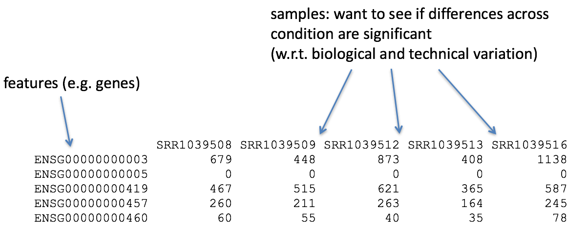
To perform differential gene expression analysis (DEA), we need to start with a matrix of counts representing the levels of gene expression. It is important to understand how the count matrix is generated, before diving into the statistical analysis.
In this lesson we will briefly discuss the RNA-processing pipeline for bulk RNA-seq, and the different steps we take to go from raw sequencing reads to a gene expression count matrix.
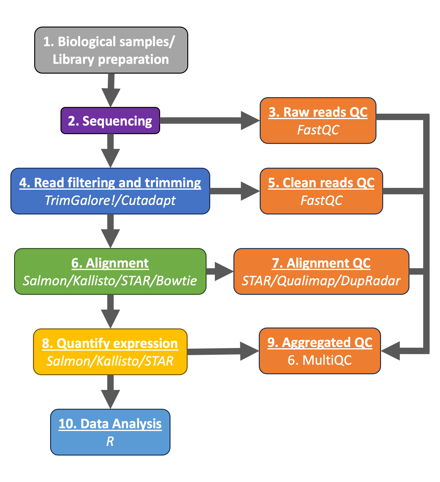
Typical RNAseq workflow
1. RNA Extraction and library preparation
Before RNA can be sequenced, it must first be extracted and separated from its cellular environment and prepared into a cDNA library. There are a number of steps involved which are outlined in the figure below, and in parallel there are various quality checks implemented to make sure we have good quality RNA to move forward with. We briefly describe some of these steps below.
a. Enriching for RNA. Once the sample has been treated with DNAse to remove any contaminating DNA sequence, the sample undergoes either selection of the mRNA (polyA selection) or depletion of the ribosomal RNA (rRNA).
Generally, rRNA represents the majority of the RNA present in a cell, while messenger RNAs represent a small percentage of total RNA, ~2% in humans. Therefore, if we want to study the protein-coding genes, we need to enrich mRNA or deplete the rRNA. For differential gene expression analysis, it is best to enrich for Poly(A)+, unless you are aiming to obtain information about long non-coding RNAs, in which case rRNA depletion is recommended.
RNA Quality check: It is essential to check the integrity of the extracted RNA prior to starting the cDNA library prepation. Traditionally, RNA integrity was assessed via gel electrophoresis by visual inspection of the ribosomal RNA bands; but that method is time consuming and imprecise. The Bioanalyzer system from Agilent will rapidly assess RNA integrity and calculate an RNA Integrity Number (RIN), which facilitates the interpretation and reproducibility of RNA quality. RIN, essentially, provides a means by which RNA quality from different samples can be compared to each other in a standardized manner.
b. Fragmentation and size selection. The remaining RNA molecules are then fragmented. This is done either via chemical, enzymatic (e.g., RNAses) or physical processes (e.g., chemical/mechanical shearing). These fragments then undergo size selection to retain only those fragments within a size range that Illumina sequencing machines can handle best, i.e., between 150 to 300 bp.
Fragment size quality check: After size selection/exclusion the fragment size distribution should be assessed to ensure that it is unimodal and well-defined.
c. Reverse transcribe RNA into double-stranded cDNA. Information about which strand a fragment originated from can be preserved by creating stranded libraries. The most commonly used method incorporates deoxy-UTP during the synthesis of the second cDNA strand (for details see Levin et al. (2010)). Once double-stranded cDNA fragments are generated, sequence adapters are ligated to the ends. (Size selection can be performed here instead of at the RNA-level.)
d. PCR amplification. If the amount of starting material is low and/or to increase the number of cDNA molecules to an amount sufficient for sequencing, libraries are usually PCR amplified. Run as few amplification cycles as possible to avoid PCR artifacts.
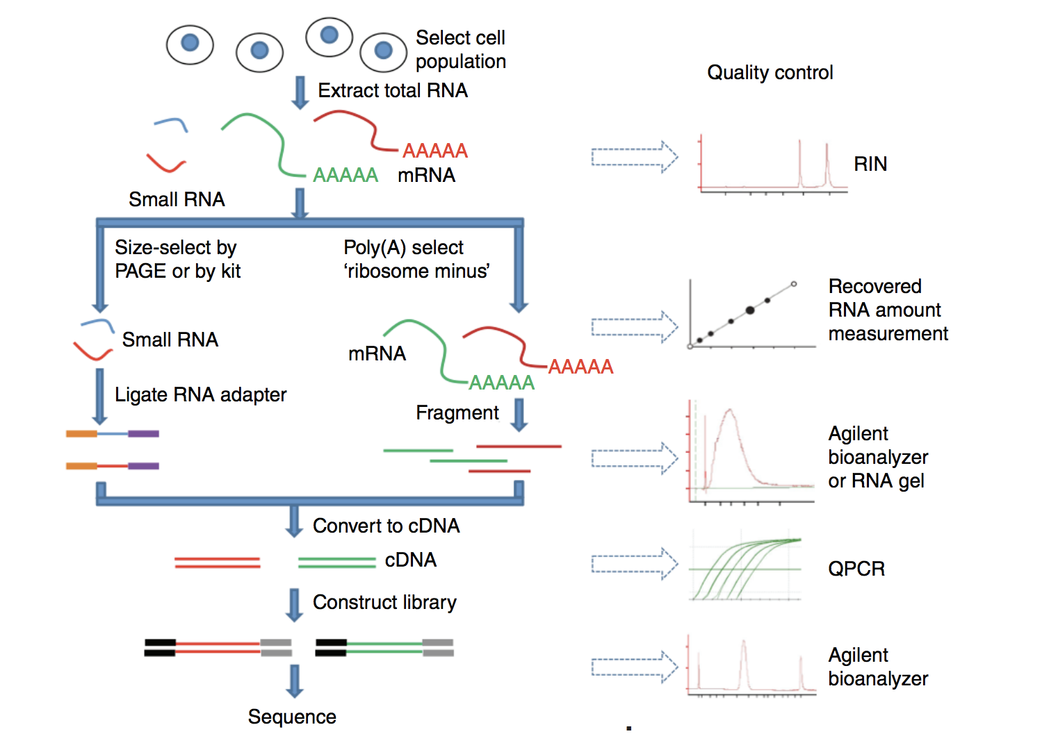
Image source: Zeng and Mortavi, 2012
2. Sequencing (Illumina)
Sequencing of the cDNA libraries will generate reads. Reads correspond to the nucleotide sequences of the ends of each of the cDNA fragments in the library. You will have the choice of sequencing either a single end of the cDNA fragments (single-end reads) or both ends of the fragments (paired-end reads).

- SE - Single end dataset => Only Read1
- PE - Paired-end dataset => Read1 + Read2
- PE can be 2 separate FastQ files or just one with interleaved pairs
Generally, single-end sequencing is sufficient unless it is expected that the reads will match multiple locations on the genome (e.g. organisms with many paralogous genes), assemblies are being performed, or for splice isoform differentiation. On the other hand, paired-end sequencing helps resolve structural genome rearrangements e.g. insertions, deletions, or inversions. Furthermore, paired reads improve the alignment/assembly of reads from repetitive regions. The downside of this type of sequencing is that it may be twice as expensive.
The scientific community is moving towards paired-end sequencing in general. However, for many purposes, single-end reads are perfectly adequate.
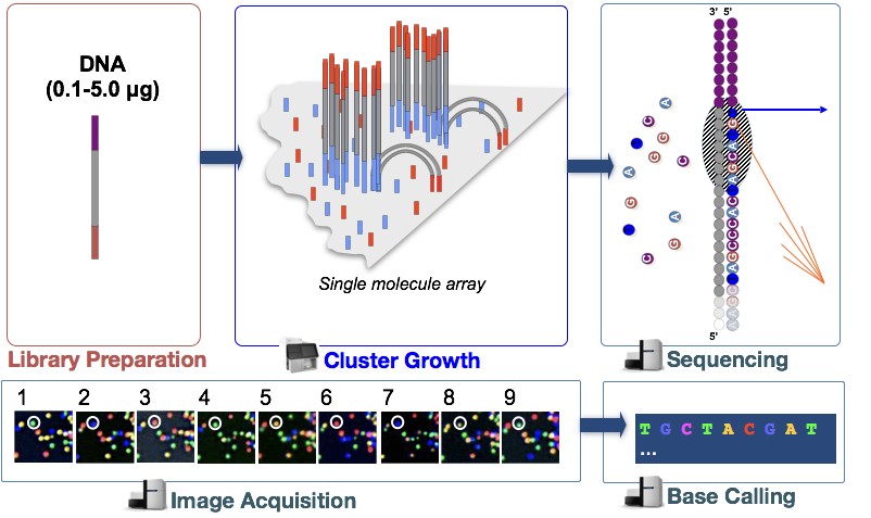
Sequencing-by-synthesis
Illumina sequencing technology uses a sequencing-by-synthesis approach. To explore sequencing by synthesis in more depth, please watch this linked video on Illumina's YouTube channel.
We have provided a brief explanation of the steps below:
- Cluster growth: The DNA fragments in the cDNA library are denatured and hybridized to the glass flowcell (adapter complementarity). Each fragment is then clonally amplified, forming a cluster of double-stranded DNA. This step is necessary to ensure that the sequencing signal will be strong enough to be detected/captured unambiguously for each base of each fragment. NOTE: Number of clusters ~= Number of reads
- Sequencing: The sequencing of the fragment ends is based on fluorophore labelled dNTPs with reversible terminator elements. In each sequencing cycle, a base is incorporated into every cluster and excited by a laser.
- Image acquisition: Each dNTP has a distinct excitatory signal emission which is captured by cameras.
- Base calling: The Base calling program will then generate the sequence of bases, i.e. reads, for each fragment/cluster by assessing the images captured during the many sequencing cycles. In addition to calling the base in every position, the base caller will also report the certainty with which it was able to make the call (quality information). NOTE: Number of sequencing cycles = Length of reads
3. Quality control of raw sequencing data
The raw reads obtained from the sequencer are stored as FASTQ files. The FASTQ file format is the de facto file format for sequence reads generated from next-generation sequencing technologies.
Each FASTQ file is a text file which represents sequence readouts for a sample. Each read is represented by 4 lines as shown below:
@HWI-ST330:304:H045HADXX:1:1101:1111:61397
CACTTGTAAGGGCAGGCCCCCTTCACCCTCCCGCTCCTGGGGGANNNNNNNNNNANNNCGAGGCCCTGGGGTAGAGGGNNNNNNNNNNNNNNGATCTTGG
+
@?@DDDDDDHHH?GH:?FCBGGB@C?DBEGIIIIAEF;FCGGI##################################################################################################################
| Line | Description |
|---|---|
| 1 | Always begins with '\@' and then information about the read |
| 2 | The actual DNA sequence, where N means that no base was called (poor quality) |
| 3 | Always begins with a '+' and sometimes the same info as in line 1 |
| 4 | Has a string of characters which represent the quality scores; must have same number of characters as line 2 |
FastQC is a commonly used software that provides a simple way to do some quality control checks on raw sequence data.
The main functions include:
- Providing a quick overview to tell you in which areas there may be problems
- Summary graphs and tables to quickly assess your data
- Export of results to an HTML based permanent report
Quality metrics
Here you will find a list of metrics that FASTQC will calculate on your reads:
- Phred Quality Scores: Preprocessed reads are evaluated based on Phred quality scores. These scores represent the estimated probability of a base call being incorrect. Higher Phred scores indicate higher base-call accuracy.
- Sequence Length Distribution: QC tools assess the length distribution of the preprocessed reads. This helps in identifying any biases introduced during preprocessing, such as excessive shortening of reads.
- Adapter Contamination: Even after preprocessing, it's crucial to confirm that all adapter sequences have been successfully removed. Any remaining adapter contamination can adversely affect downstream analyses.
- GC Content: Evaluating the GC content of preprocessed reads helps in detecting biases that might have been introduced during library preparation or sequencing.
- Duplicate Reads: Preprocessed reads should be checked for duplicates. Duplicate reads can arise due to PCR amplification biases during library preparation.
- K-mer Content: QC tools can analyze the frequency distribution of k-mers (short sequences of length k). Deviations from the expected k-mer distribution may indicate biases or contamination.
- Overall Sequence Quality: A summary of the overall quality metrics, including mean Phred scores, per-base sequence quality, and sequence duplication levels, provides a comprehensive assessment of data quality.
4. Read filtering and trimming
The reads in a FASTQ file may contain errors, low-quality bases and adapter sequences. To extract reliable biological information, it's crucial to preprocess or "clean" this data through trimming and filtering.
Trimming involves the removal of low-quality bases from the ends of reads. Low-quality bases can arise due to various factors, such as limitations in the sequencing technology or degradation during sample preparation. Trimming helps to improve the overall quality of the data, which is essential for downstream analysis.
Additionally, adapter sequences, which are short DNA sequences used in library preparation, can be mistakenly sequenced along with the target DNA. Trimming these adapters is necessary to ensure accurate alignment and subsequent analysis.
Filtering is a broader process that involves the removal of reads that do not meet specific quality criteria. For example, reads with an excessive number of low-quality bases or those that are too short may be discarded. This step helps to retain high-confidence data for downstream analysis.
Trimming and filtering are crucial steps in NGS data processing because they improve the accuracy and reliability of the data. Without these steps, subsequent analyses like genome assembly, variant calling, and transcript quantification can be severely affected. By reducing noise and removing artifacts, researchers can obtain a clearer and more accurate picture of the biological information encoded in the sequencing data.
To trim and filter reads, we can use bioinformatics tools such as like Cutadapt and Trim Galore. They offer powerful and versatile functionalities for trimming and filtering raw sequencing reads, ensuring that only high-quality data is used for subsequent analyses.
Cutadapt
Cutadapt is a widely-used and highly flexible tool designed specifically for removing adapter sequences from NGS reads. Adapter sequences can be introduced during library preparation and may subsequently be sequenced along with the target DNA or RNA. Cutadapt employs a sophisticated algorithm to accurately and efficiently identify and trim these adapters.
Key features of Cutadapt include:
- Adapter Detection and Removal: Cutadapt can detect and remove adapters with high precision, even in cases where the adapter sequence is only partially known.
- Error-Tolerant Matching: It can perform error-tolerant matching, allowing it to handle cases where adapter sequences might have minor variations or mutations.
- Quality Trimming: Cutadapt can also perform quality trimming, which involves removing low-quality bases from the ends of reads. This feature helps in improving data quality.
- Batch Processing: It can process multiple files in a single run, making it efficient for handling large-scale datasets.
- Format Compatibility: Cutadapt supports various file formats commonly used in NGS, such as FASTQ and SAM.
Trim Galore
Trim Galore is a user-friendly wrapper script that combines the functionalities of Cutadapt with FastQC, to provide a streamlined solution for trimming and quality control of NGS data. It simplifies the preprocessing workflow by automating the process of running Cutadapt and generating quality reports through FastQC.
5. Quality control of clean sequencing data
After preprocessing the reads, we assess again the quality and reliability of the sequencing reads. This QC step is essential to ensure that only high-quality data is used for downstream analyses. We will check that the quality metrics calculated on the raw reads have improved:
- Improved Quality: Preprocessed reads typically exhibit higher quality scores and improved base call accuracy compared to raw reads. This is because preprocessing steps like adapter trimming and quality filtering remove low-quality bases and artifacts.
- Reduced Noise and Artifacts: Preprocessing removes noise, such as adapter sequences, low-quality bases, and sequencing errors. This leads to cleaner data, enhancing the accuracy of downstream analyses.
6. Alignment
After checking that the quality of our reads is adequate, we can proceed to aligning our sequencing reads to a reference genome. By doing this, we can identify variations, quantify gene expression levels and study other genomic features. For the purposes of this workshop, we are mostly interested in the ability to quantify gene expression levels for our differential expression analysis.
Alignment is achieved by finding the best matching position in the reference genome for each read. This is a computationally intensive task due to the vast amount of data generated by NGS experiments. Alignment tools utilize various algorithms and techniques to efficiently perform this task, which can be mostly divided in two categories: traditional aligment and pseudoaligment.
Traditional alignment tools
Traditional alignment consists in the process described above, matching your preprocessed reads to a reference genome. This process involves determining the genomic location from which each read originated. The result of the alignment will be a SAM/BAM file, which will contain information regarding the quality and the genomic position of the aligned read.
Below we will highlight some of the most common alignment algorithms:
Bowtie2
Bowtie2 is a widely-used, ultra-fast alignment tool designed for aligning short reads (typically from Illumina platforms) to a reference genome. It employs a Burrows-Wheeler transform-based algorithm, which allows it to quickly and accurately align millions of reads. Bowtie is highly efficient, making it a popular choice for large-scale NGS projects.
STAR
STAR (Spliced Transcripts Alignment to a Reference) is a specialized alignment tool tailored for RNA-Seq data. It is designed to align reads to a reference genome, taking into account the splicing events that occur in eukaryotic genomes. STAR can align both short and long RNA-Seq reads, making it a versatile tool for gene expression analysis and transcriptome mapping.
HISAT2
HISAT2 (Hierarchical Indexing for Spliced Alignment of Transcripts) is another prominent alignment tool widely used for aligning RNA-Seq reads to a reference genome. It employs a hierarchical indexing approach that enables efficient and accurate alignment, particularly in the presence of spliced alignments. HISAT2 is known for its speed and sensitivity, making it a popular choice for transcriptome analysis. It also offers the advantage of reduced memory usage compared to some other alignment tools, making it suitable for a wide range of computational environments. HISAT2's ability to accurately handle splice junctions makes it a valuable tool for studying alternative splicing events and other complex features of transcriptomes.
Pseudoalignment
Pseudoalignment is a concept in computational biology and genomics that offers an alternative approach to traditional read alignment. Unlike traditional alignment, which involves finding the exact position of a read within a reference genome, pseudoalignment estimates the likelihood that a read originates from a specific transcript or set of transcripts without explicitly mapping it to the reference genome.
Pseudoalignment tools, like Salmon and Kallisto, achieve this by building an index of transcript sequences rather than the entire genome. They use efficient algorithms to quickly determine which transcripts are likely to be the source of a given read. This approach significantly reduces the computational resources required for quantifying gene expression, as it circumvents the need to align every read to the entire genome. By focusing on transcripts, pseudoalignment provides a faster and more memory-efficient solution, making it especially advantageous for large-scale RNA-Seq studies and in situations where rapid quantification of gene expression levels is critical, such as in time-sensitive experiments or in scenarios with limited computational resources.
Pseudoalignment is well-suited for studying gene expression in well-annotated genomes, where the transcriptome is relatively well-characterized, although not so great with other under-studied organisms. We will highlight a couple of these algorithms below.
Salmon
Salmon uses a lightweight and rapid algorithm based on the concept of selective alignment. It directly quantifies transcript abundance without explicitly aligning reads to the reference genome. This makes Salmon especially efficient for large-scale RNA-Seq studies, where speed and accuracy are crucial.
Kallisto
Similar to Salmon, Kallisto employs a pseudoalignment strategy. It quantifies transcript abundance by estimating the compatibility of reads with known transcripts, bypassing the need for full alignment to the genome. This approach makes Kallisto extremely fast, making it an attractive choice for rapid and accurate gene expression quantification.
7. Quality control of aligned reads
After aligning our reads, it is essential to perform some basic quality checks on the sequencing data. However, this step is only possible if you align your reads using a traditional algorithm, since pseudoaligment tools will not create a BAM file that can be checked for quality control.
Qualimap
A tool called Qualimap explores the features of aligned reads in the context of the genomic region they map to, hence providing an overall view of the data quality (as an HTML file). Various quality metrics assessed by Qualimap include:
- DNA or rRNA contamination
- 5'-3' biases
- Coverage biases
dupRadar
The [dupRadar[(https://bioconductor.org/packages/release/bioc/vignettes/dupRadar/inst/doc/dupRadar.html) package provides an assessment of the level of duplication of your reads, allowing you to distinguish PCR amplification artifacts from true biological signals.
The number of reads per base assigned to a gene in an ideal RNA-Seq data set is expected to be proportional to the abundance of its transcripts in the sample. For lowly expressed genes we expect read duplication to happen rarely by chance, while for highly expressed genes - depending on the total sequencing depth - we expect read duplication to happen often.
A good way to learn if a dataset is following this trend is by relating the normalized number of counts per gene (RPK, as a quantification of the gene expression) and the fraction represented by duplicated reads. For example, the plots below show very well how duplicates should look in a good experiment (left) compared to another experiment with duplication issues(right)

8. Quantify expression
Once we have explored the quality of our raw reads, we can move on to quantifying expression at the transcript level. The goal of this step is to identify from which transcript each of the reads originated from and the total number of reads associated with each transcript.
Quantification from BAM files is the traditional method of estimating gene expression levels. It involves aligning reads to a reference genome using tools like Bowtie, STAR, or HISAT2, and then counting the number of reads that map to each gene or transcript. This process relies on the generation of a BAM (Binary Alignment/Map) file, which records the alignment information for each read. Quantification tools like featureCounts or HTSeq then process the BAM file to count reads that align to each annotated gene.
Pseudoaligment tools such as Kallisto and Salmon they perform pseudoalignment and quantification in the same step by quickly mapping reads to a set of reference transcripts. This is done using an indexing strategy that efficiently assigns reads to potential transcript sources. Pseudoquantification is particularly fast and memory-efficient, making it ideal for large-scale transcriptome studies. It provides accurate estimates of transcript abundance, even in the presence of complex transcript structures.
In this course, we will use the expression estimates, often referred to as 'pseudocounts', obtained from Salmon as the starting point for the differential gene expression analysis.
9. Aggregation of quality control checks
Throughout the workflow we have performed various steps of quality checks on our data. You will need to do this for every sample in your dataset, making sure these metrics are consistent across the samples for a given experiment. Outlier samples should be flagged for further investigation and potential removal.
Manually tracking these metrics and browsing through multiple HTML reports (FastQC, Qualimap) and log files (Salmon, STAR) for each sample is tedious and prone to errors. MultiQC is a tool which aggregates results from several tools and generates a single HTML report with plots to visualize and compare various QC metrics between the samples. Assessment of the QC metrics may result in the removal of samples before proceeding to the next step, if necessary.
Once the QC has been performed on all the samples, we are ready to get started with Differential Gene Expression analysis with DESeq2!
This lesson was originally developed by members of the teaching team at the Harvard Chan Bioinformatics Core (Meeta Mistry, Radhika Khetani and Mary Piper) (HBC).
Created: November 28, 2023