DESeq2: Model fitting and Hypothesis testing
Last updated: November 28, 2023
Section Overview
🕰 Time Estimation: 90 minutes
💬 Learning Objectives:
- Demonstrate the use of the design formula with simple and complex designs
- Construct R code to execute the differential expression analysis workflow with DESeq2
- Describe the process of model fitting
- Compare two methods for hypothesis testing (Wald test vs. LRT)
- Discuss the steps required to generate a results table for pairwise comparisons (Wald test)
- Recognize the importance of multiple test correction
- Identify different methods for multiple test correction
- Summarize the different levels of gene filtering
- Evaluate the number of differentially expressed genes produced for each comparison
- Construct R objects containing significant genes from each comparison
The final step in the DESeq2 workflow is taking the counts for each gene and fitting it to the model and testing for differential expression.
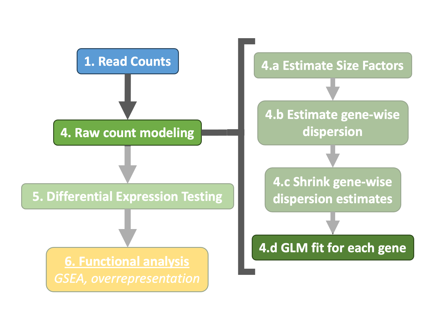
Generalized Linear Model
As described earlier, the count data generated by RNA-seq exhibits overdispersion (variance > mean) and the statistical distribution used to model the counts needs to account for this. As such, DESeq2 uses a negative binomial distribution to model the RNA-seq counts using the equation below:
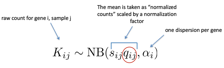
The two parameters required are the size factor, and the dispersion estimate. Next, a generalized linear model (GLM) of the NB family is used to fit the data. Modeling is a mathematically formalized way to approximate how the data behaves given a set of parameters.
About GLMs
"In statistics, the generalized linear model (GLM) is a flexible generalization of ordinary linear regression that allows for response variables that have error distribution models other than a normal distribution. The GLM generalizes linear regression by allowing the linear model to be related to the response variable via a link function and by allowing the magnitude of the variance of each measurement to be a function of its predicted value." (Wikipedia).
After the model is fit, coefficients are estimated for each sample group along with their standard error. The coefficients are the estimates for the log2 fold changes, and will be used as input for hypothesis testing.
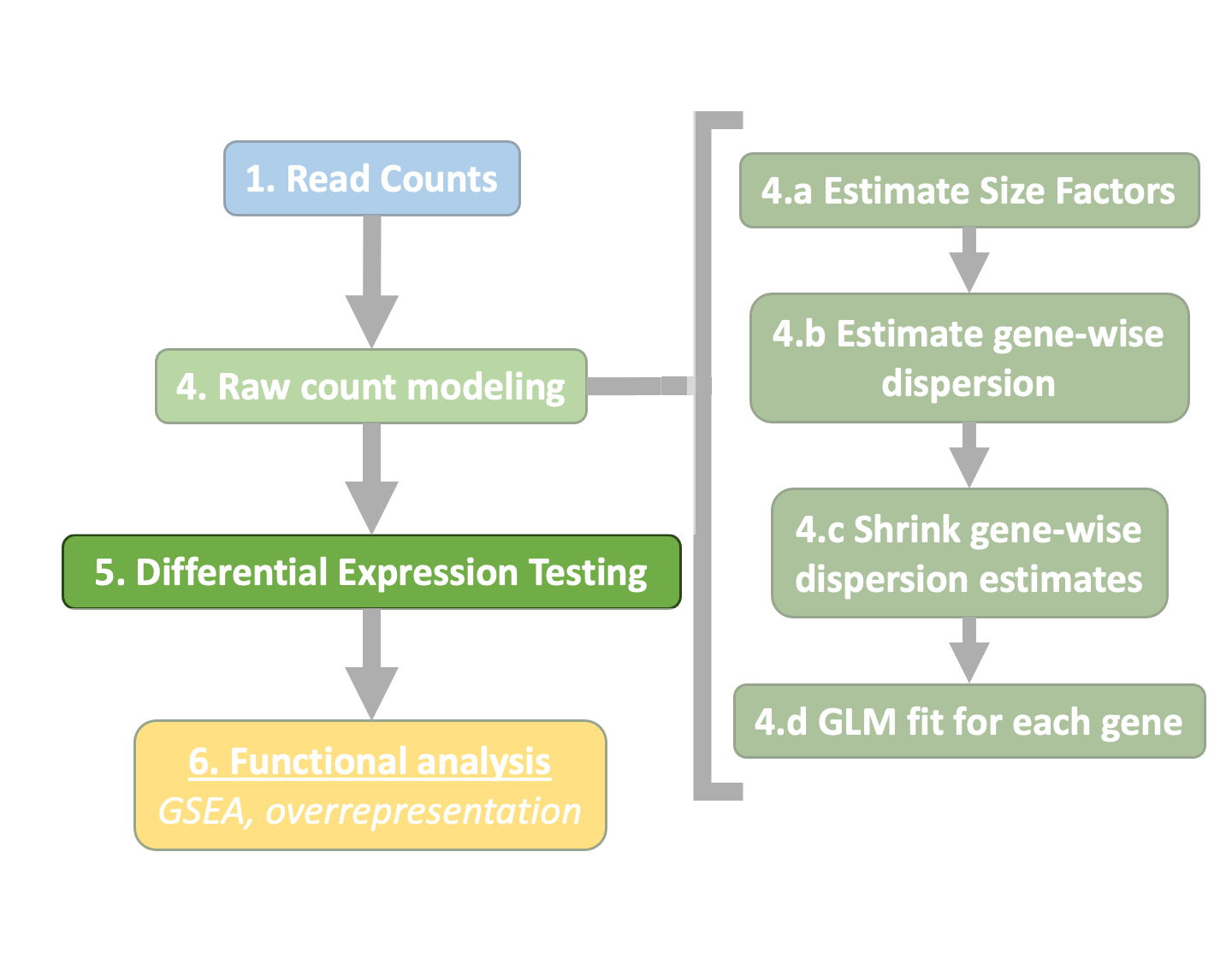
Hypothesis testing
The first step in hypothesis testing is to set up a null hypothesis for each gene. In our case, the null hypothesis is that there is no differential expression across the two sample groups (LFC == 0). Notice that we can do this without observing any data, because it is based on a thought experiment. Second, we use a statistical test to determine if based on the observed data, the null hypothesis can be rejected.
Wald test
In DESeq2, the Wald test is the default used for hypothesis testing when comparing two groups. The Wald test is a test usually performed on parameters that have been estimated by maximum likelihood. In our case we are testing each gene model coefficient (LFC) which was derived using parameters like dispersion, which were estimated using maximum likelihood.
DESeq2 implements the Wald test by:
- Taking the LFC and dividing it by its standard error, resulting in a z-statistic.
- The z-statistic is compared to a standard normal distribution, and a p-value is computed reporting the probability that a z-statistic at least as extreme as the observed value would be selected at random.
- If the p-value is small we reject the null hypothesis and state that there is evidence against the null (i.e. the gene is differentially expressed).
The model fit and Wald test were already run previously as part of the DESeq() function:
## DO NOT RUN THIS CODE

## Create DESeq2Dataset object
dds <- DESeqDataSetFromTximport(txi,
                                   colData = meta %>% column_to_rownames("sample"),
                              design = ~ condition)
## Run analysis
dds <- DESeq(dds)
Likelihood ratio test (LRT)
An alternative to pair-wise comparisons is to analyze all levels of a factor at once. By default, the Wald test is used to generate the results table, but DESeq2 also offers the LRT which is used to identify any genes that show change in expression across the different levels. This type of test can be especially useful in analyzing time course experiments.
LRT vs Wald test
The Wald test evaluates whether a gene's expression is up- or down-regulated in one group compared to another, while the LRT identifies genes that are changing in expression in any combination across the different sample groups. For example:
- Gene expression is equal between Control and Vampirium, but is less in Garlicum
- Gene expression of Vampirium is lower than Control and Control is lower than Garlicum
- Gene expression of Garlicum is equal to Control, but less than Vampirium.
Using LRT, we are evaluating the null hypothesis that the full model fits just as well as the reduced model. If we reject the null hypothesis, this suggests that there is a significant amount of variation explained by the full model (and our main factor of interest), therefore the gene is differentially expressed across the different levels. Generally, this test will result in a larger number of genes than the individual pair-wise comparisons. However, while the LRT is a test of significance for differences of any level of the factor, one should not expect it to be exactly equal to the union of sets of genes using Wald tests (although we do expect a majority overlap).
To use the LRT, we use the DESeq() function but this time adding two arguments:
- specifying that we want to use the LRT test
- the "reduced" model
# The full model was specified previously with the `design = ~ condition`:
# dds <- DESeqDataSetFromTximport(txi,
                                   # colData = meta %>% column_to_rownames("sample"),
                              # design = ~ condition)

# Likelihood ratio test
dds_lrt <- DESeq(dds, test="LRT", reduced = ~ 1)
Since our "full" model only has one factor (sampletype), the "reduced" model (removing that factor) is just the intercept (~ 1). You will find that similar columns are reported for the LRT test. One thing to note is, even though there are fold changes present they are not directly associated with the actual hypothesis test.
Time course analysis with LTR
The LRT test can be especially helpful when performing time course analyses. We can use the LRT to explore whether there are any significant differences in treatment effect between any of the timepoints.
For have an experiment looking at the effect of treatment over time on mice of two different genotypes. We could use a design formula for our "full model" that would include the major sources of variation in our data: genotype, treatment, time, and our main condition of interest, which is the difference in the effect of treatment over time (treatment:time).
To perform the LRT test, we can determine all genes that have significant differences in expression between treatments across time points by giving the "reduced model" without the treatment:time term:
Then, we could run our test by using the following code:
dds_lrt <- DESeqDataSetFromMatrix(countData = data, colData = metadata, design = ~ genotype + treatment + time + treatment:time)

dds_lrt_time <- DESeq(dds_lrt, test="LRT", reduced = ~ genotype + treatment + time)
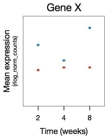
This analysis will not return genes where the treatment effect does not change over time, even though the genes may be differentially expressed between groups at a particular time point, as shown in the figure below:
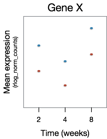
The significant DE genes will represent those genes that have differences in the effect of treatment over time, an example is displayed in the figure below:
Multiple test correction
Regardless of whether we use the Wald test or the LRT, each gene that has been tested will be associated with a p-value. It is this result which we use to determine which genes are considered significantly differentially expressed. However, we cannot use the p-value directly.
What does the p-value mean?
A gene with a significance cut-off of p \< 0.05, means there is a 5% chance it is a false positive. For example, if we test 20,000 genes for differential expression, at p \< 0.05 we would expect to find 1,000 DE genes by chance. If we found 3000 genes to be differentially expressed total, roughly one third of our genes are false positives! We would not want to sift through our "significant" genes to identify which ones are true positives.
Since each p-value is the result of a single test (single gene). The more genes we test, the more we inflate the false positive rate. This is the multiple testing problem.
Correcting the p-value for multiple testing
There are a few common approaches for multiple test correction:
- Bonferroni: The adjusted p-value is calculated by: \(p-value*m\) (\(m\) = total number of tests). This is a very conservative approach with a high probability of false negatives, so is generally not recommended.
- FDR/Benjamini-Hochberg: Benjamini and Hochberg (1995) defined the concept of False Discovery Rate (FDR) and created an algorithm to control the expected FDR below a specified level given a list of independent p-values. More info about BH.
- Q-value / Storey method: The minimum FDR that can be attained when calling that feature significant. For example, if gene X has a q-value of 0.013 it means that 1.3% of genes that show p-values at least as small as gene X are false positives.
DESeq2 helps reduce the number of genes tested by removing those genes unlikely to be significantly DE prior to testing, such as those with low number of counts and outlier samples (see below). However, multiple test correction is also implemented to reduce the False Discovery Rate using an interpretation of the Benjamini-Hochberg procedure.
So what does FDR \< 0.05 mean?
By setting the FDR cutoff to < 0.05, we're saying that the proportion of false positives we expect amongst our differentially expressed genes is 5%. For example, if you call 500 genes as differentially expressed with an FDR cutoff of 0.05, you expect 25 of them to be false positives.
Exploring Results (Wald test)
By default DESeq2 uses the Wald test to identify genes that are differentially expressed between two sample groups. Given the factor(s) used in the design formula, and how many factor levels are present, we can extract results for a number of different comparisons. Here, we will walk you through how to obtain results from the dds object and provide some explanations on how to interpret them.
Wald test on continuous variables
The Wald test can also be used with continuous variables. If the variable of interest provided in the design formula is continuous-valued, then the reported log2FoldChange is per unit of change of that variable.
Specifying contrasts
In our dataset, we have three sample groups so we can make three possible pairwise comparisons:
- Control vs. Vampirium
- Garlicum vs. Vampirium
- Garlicum vs. Control
We are really only interested in 1 and 2 from above. When we initially created our dds object we had provided ~ condition as our design formula, indicating that sampletype is our main factor of interest.
To indicate which two sample groups we are interested in comparing, we need to specify contrasts. The contrasts are used as input to the DESeq2 results() function to extract the desired results.
Contrasts can be specified in three different ways:
1.Contrasts can be supplied as a character vector with exactly three elements: the name of the factor (of interest) in the design formula, the name of the two factors levels to compare. The factor level given last is the base level for the comparison. The syntax is given below:
# DO NOT RUN!
contrast <- c("condition", "level_to_compare", "base_level")
results(dds, contrast = contrast)
2.Contrasts can be given as a list of 2 character vectors: the names of the fold changes for the level of interest, and the names of the fold changes for the base level. These names should match identically to the elements of resultsNames(object). This method can be useful for combining interaction terms and main effects.
# DO NOT RUN!
resultsNames(dds) # to see what names to use
contrast <- list(resultsNames(dds)[1], resultsNames(dds)[2])
results(dds, contrast = contrast)
3.One of the results from resultsNames(dds) and the name argument. This one is the simplest but it can also be very restrictive:
# DO NOT RUN!
resultsNames(dds) # to see what names to use
results(dds, name = resultsNames(dds)[2])
Alternatively, if you only had two factor levels you could do nothing and not worry about specifying contrasts (i.e. results(dds)). In this case, DESeq2 will choose what your base factor level based on alphabetical order of the levels.
To start, we want to evaluate expression changes between the control samples and the vampirium samples. As such we will use the first method for specifying contrasts and create a character vector:
Exercise 1
Define contrasts for Vampirium samples using one of the two methods above.
Solution to Exercise 1
First let's check the metadata:
Since we have only given the condition column in the design formula, the first element should be condition. The second element is the condition we are interested, control and our base level is vampirium.
Does it matter what I choose to be my base level?
Yes, it does matter. Deciding what level is the base level will determine how to interpret the fold change that is reported. So for example, if we observe a log2 fold change of -2 this would mean the gene expression is lower in factor level of interest relative to the base level. Thus, if leaving it up to DESeq2 to decide on the contrasts be sure to check that the alphabetical order coincides with the fold change direction you are anticipating.
The results table
Now that we have our contrast created, we can use it as input to the results() function. Let's take a quick look at the help manual for the function:
You will see we have the option to provide a wide array of arguments and tweak things from the defaults as needed. As we go through the lesson we will keep coming back to the help documentation to discuss some arguments that are good to know about.
## Extract results for Control vs Vampirium samples
res_tableCont <- results(dds, contrast=contrast_cont, alpha = 0.05)
Warning
For our analysis, in addition to the contrast argument we will also provide a value of 0.05 for the alpha argument. We will describe this in more detail when we talk about gene-level filtering.
The results table that is returned to us is a DESeqResults object, which is a simple subclass of DataFrame. In many ways it can be treated like a dataframe (i.e when accessing/subsetting data), however it is important to recognize that there are differences for downstream steps like visualization.
Now let's take a look at what information is stored in the results:
We have six columns of information reported for each gene (row). We can use the mcols() function to extract information on what the values stored in each column represent:
baseMean: mean of normalized counts for all sampleslog2FoldChange: log2 fold changelfcSE: standard errorstat: Wald statisticpvalue: Wald test p-valuepadj: BH adjusted p-values
p-values
The p-value is a probability value used to determine whether there is evidence to reject the null hypothesis. A smaller p-value means that there is stronger evidence in favor of the alternative hypothesis.
The padj column in the results table represents the p-value adjusted for multiple testing, and is the most important column of the results. Typically, a threshold such as padj \< 0.05 is a good starting point for identifying significant genes. The default method for multiple test correction in DESeq2 is the FDR. Other methods can be used with the pAdjustMethod argument in the results() function.
Gene-level filtering
Let's take a closer look at our results table. As we scroll through it, you will notice that for selected genes there are NA values in the pvalue and padj columns. What does this mean?
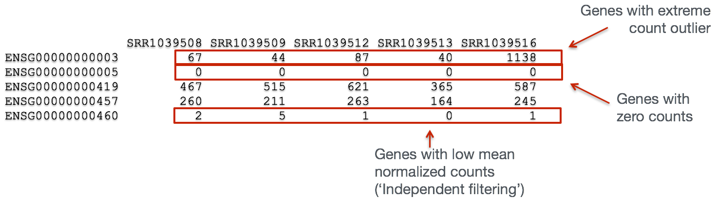
The missing values represent genes that have undergone filtering as part of the DESeq() function. Prior to differential expression analysis it is beneficial to omit genes that have little or no chance of being detected as differentially expressed. This will increase the power to detect differentially expressed genes. DESeq2 does not physically remove any genes from the original counts matrix, and so all genes will be present in your results table. The genes omitted by DESeq2 meet one of the three filtering criteria outlined below:
1. Genes with zero counts in all samples
If within a row, all samples have zero counts there is no expression information and therefore these genes are not tested. In our case, there are no genes that fulfill this criteria, since we have already filtered out these genes ourselves when we created our dds object.
# Show genes with zero expression
res_tableCont %>%
  as_tibble(rownames = "gene") %>%
  dplyr::filter(baseMean==0) %>%
  head()
Info
If there would be any genes meeting this criteria, the baseMean column for these genes will be zero, and the log2 fold change estimates, p-value and adjusted p-value will all be set to NA.
2. Genes with an extreme count outlier
The DESeq() function calculates, for every gene and for every sample, a diagnostic test for outliers called Cook's distance. Cook's distance is a measure of how much a single sample is influencing the fitted coefficients for a gene, and a large value of Cook's distance is intended to indicate an outlier count. Genes which contain a Cook's distance above a threshold are flagged, however at least 3 replicates are required for flagging, as it is difficult to judge which sample might be an outlier with only 2 replicates. We can turn off this filtering by using the cooksCutoff argument in the results() function.
# Show genes that have an extreme outlier
res_tableCont %>%
  as_tibble(rownames = "gene") %>%
  dplyr::filter(is.na(pvalue) & is.na(padj) & baseMean > 0) %>%
  head()
It seems that we have some genes with outliers!
Info
If a gene contains a sample with an extreme count outlier then the p-value and adjusted p-value will be set to NA.
3. Genes with a low mean normalized counts
DESeq2 defines a low mean threshold, that is empirically determined from your data, in which the fraction of significant genes can be increased by reducing the number of genes that are considered for multiple testing. This is based on the notion that genes with very low counts are not likely to see significant differences typically due to high dispersion.
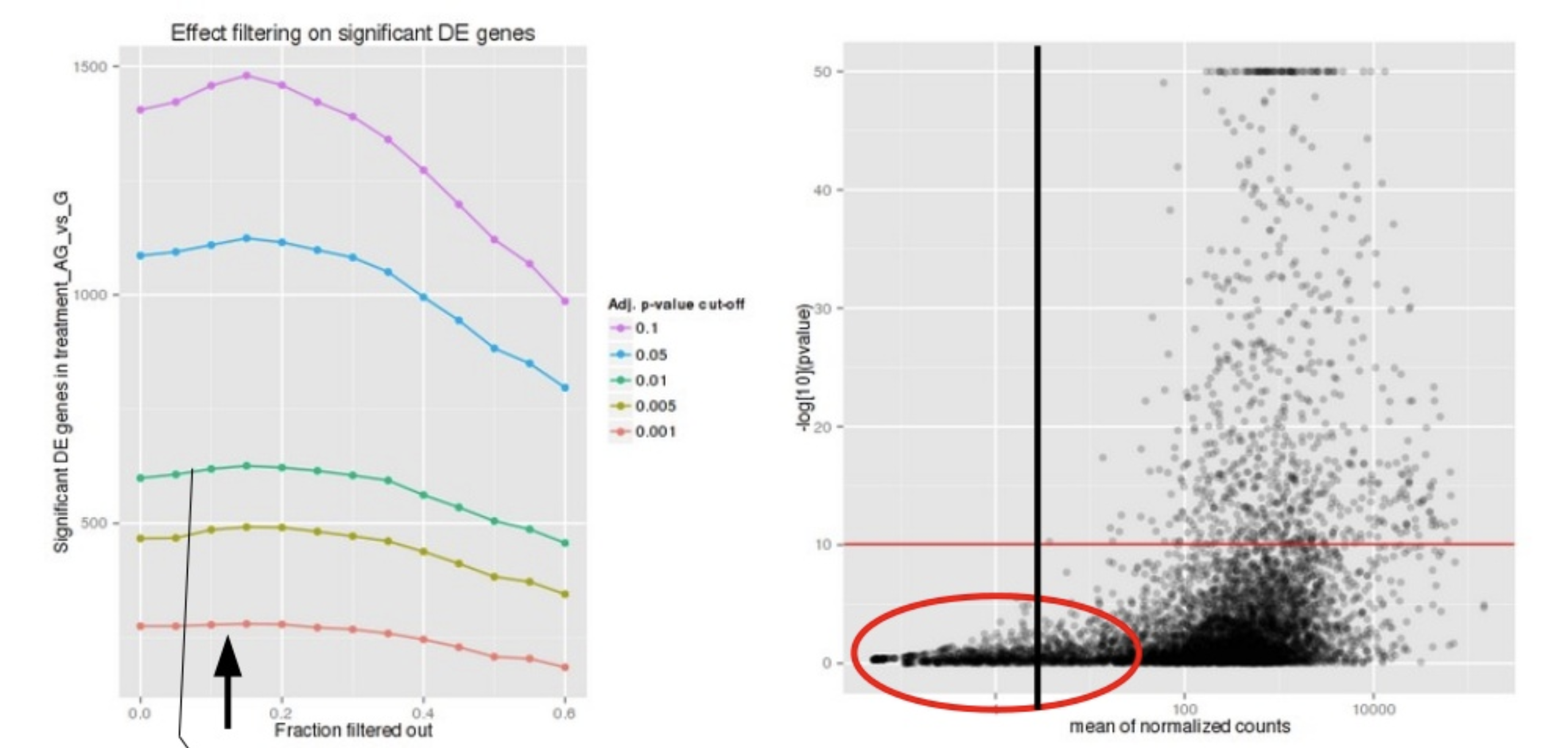
Image courtesy of slideshare presentation from Joachim Jacob, 2014.
At a user-specified value (alpha = 0.05), DESeq2 evaluates the change in the number of significant genes as it filters out increasingly bigger portions of genes based on their mean counts, as shown in the figure above. The point at which the number of significant genes reaches a peak is the low mean threshold that is used to filter genes that undergo multiple testing. There is also an argument to turn off the filtering off by setting independentFiltering = F.
# Filter genes below the low mean threshold
res_tableCont %>%
  as_tibble(rownames = "gene") %>%
  dplyr::filter(!is.na(pvalue) & is.na(padj) & baseMean > 0) %>%
  head()
Info
If a gene is filtered by independent filtering, then only the adjusted p-value will be set to NA.
Warning
DESeq2 will perform the filtering outlined above by default; however other DE tools, such as EdgeR will not. Filtering is a necessary step, even if you are using limma-voom and/or edgeR's quasi-likelihood methods. Be sure to follow pre-filtering steps when using other tools, as outlined in their user guides found on Bioconductor as they generally perform much better.*
Fold changes
Another important column in the results table, is the log2FoldChange. With large significant gene lists it can be hard to extract meaningful biological relevance. To help increase stringency, one can also add a fold change threshold. Keep in mind when setting that value that we are working with log2 fold changes, so a cutoff of log2FoldChange \< 1 would translate to an actual fold change of 2.
An alternative approach to add the fold change threshold
The results() function has an option to add a fold change threshold using the lfcThreshold argument. This method is more statistically motivated, and is recommended when you want a more confident set of genes based on a certain fold-change. It actually performs a statistical test against the desired threshold, by performing a two-tailed test for log2 fold changes greater than the absolute value specified. The user can change the alternative hypothesis using altHypothesis and perform two one-tailed tests as well. This is a more conservative approach, so expect to retrieve a much smaller set of genes!
The fold changes reported in the results table are the coefficients calculated in the GLM mentioned in the previous section.
Summarizing results
To summarize the results table, a handy function in DESeq2 is summary(). Confusingly it has the same name as the function used to inspect data frames. This function, when called with a DESeq results table as input, will summarize the results using a default threshold of padj \< 0.1. However, since we had set the alpha argument to 0.05 when creating our results table threshold: FDR \< 0.05 (padj/FDR is used even though the output says p-value < 0.05). Let's start with the OE vs control results:
In addition to the number of genes up- and down-regulated at the default threshold, the function also reports the number of genes that were tested (genes with non-zero total read count), and the number of genes not included in multiple test correction due to a low mean count.
Extracting significant differentially expressed genes
Let's first create variables that contain our threshold criteria. We will only be using the adjusted p-values in our criteria:
We can easily subset the results table to only include those that are significant using the dplyr::filter() function, but first we will convert the results table into a tibble:
# Create a tibble of results and add gene IDs to new object
res_tableCont_tb <- res_tableCont %>%
  as_tibble(rownames = "gene") %>%
  relocate(gene, .before = baseMean)

head(res_tableCont_tb)
Now we can subset that table to only keep the significant genes using our pre-defined thresholds:
# Subset the tibble to keep only significant genes
sigCont <- res_tableCont_tb %>%
  dplyr::filter(padj < padj.cutoff)
Now that we have extracted the significant results, we are ready for visualization!
Exercise 2
Vampirium Differential Expression Analysis: Garlicum versus Vampirium
Now that we have results for the Control vs Vampirium results, do the same for the Garlicum vs Vampirium samples.
- Create a contrast vector called
contrast_gar. - Use contrast vector in the
results()to extract a results table and store that to a variable calledres_tableGar. - Using a p-adjusted threshold of 0.05 (
padj.cutoff < 0.05), subsetres_tableGarto report the number of genes that are up- and down-regulated in garlicum compared to vampirium. - How many genes are differentially expressed in the Garlicum compared to Vampirium? How does this compare to the Control vs Vampirium significant gene list (in terms of numbers)?
Solutions to Exercise 2
- Contrast for Garlicum vs Vampirium
- Extract results
- Significant genes
padj.cutoff <- 0.05
sigGar <- res_tableGar %>% as_tibble(rownames = "gene") %>%
  relocate(gene, .before = baseMean) %>% dplyr::filter(padj < padj.cutoff)
- Comparison against sigGar vs sigCont
nrow(sigGar) #number of significant genes in Garlicum vs Vampirium
nrow(sigCont) #number of significant genes in Control vs Vampirium
sigCont has almost 2000 more genes that are differentially expressed!
This lesson was originally developed by members of the teaching team (Mary Piper, Meeta Mistry, Radhika Khetani) at the Harvard Chan Bioinformatics Core (HBC).
Some materials and hands-on activities were adapted from RNA-seq workflow on the Bioconductor website
Created: November 28, 2023