Functional class scoring
Last updated: November 28, 2023
Section Overview
🕰 Time Estimation: 40 minutes
💬 Learning Objectives:
- Discuss functional class scoring, and pathway topology methods
- Construct a GSEA analysis using GO and KEGG gene sets
- Examine results of a GSEA using pathview package
- List other tools and resources for identifying genes of novel pathways or networks
Over-representation analysis is only a single type of functional analysis method that is available for teasing apart the biological processes important to your condition of interest. Other types of analyses can be equally important or informative, including functional class scoring methods.
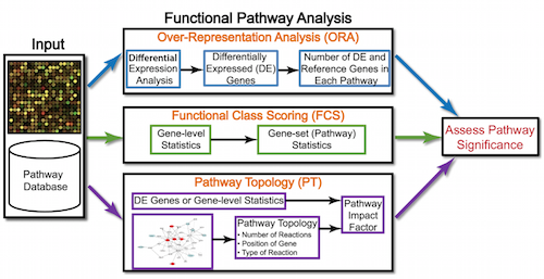
Functional class scoring (FCS) tools, such as GSEA, most often use the gene-level statistics or log2 fold changes for all genes from the differential expression results, then look to see whether gene sets for particular biological pathways are enriched among the large positive or negative fold changes.
The hypothesis of FCS methods is that although large changes in individual genes can have significant effects on pathways (and will be detected via ORA methods), weaker but coordinated changes in sets of functionally related genes (i.e., pathways) can also have significant effects. Thus, rather than setting an arbitrary threshold to identify 'significant genes', all genes are considered in the analysis. The gene-level statistics from the dataset are aggregated to generate a single pathway-level statistic and statistical significance of each pathway is reported. This type of analysis can be particularly helpful if the differential expression analysis only outputs a small list of significant DE genes.
Gene set enrichment analysis using clusterProfiler and Pathview
Using the log2 fold changes obtained from the differential expression analysis for every gene, gene set enrichment analysis and pathway analysis can be performed using clusterProfiler and Pathview tools.
For a gene set or pathway analysis using clusterProfiler, coordinated differential expression over gene sets is tested instead of changes of individual genes.
Info
Gene sets are pre-defined groups of genes, which are functionally related. Commonly used gene sets include those derived from KEGG pathways, Gene Ontology terms, MSigDB, Reactome, or gene groups that share some other functional annotations, etc. Consistent perturbations over such gene sets frequently suggest mechanistic changes.
Preparation for GSEA
clusterProfiler offers several functions to perform GSEA using different genes sets, including but not limited to GO, KEGG, and MSigDb. We will use the KEGG gene sets, which identify genes using their Entrez IDs. Therefore, to perform the analysis, we will need to acquire the Entrez IDs. We will also need to remove the Entrez ID NA values and duplicates (due to gene ID conversion) prior to the analysis:
# Remove any NA values (reduces the data by quite a bit) and duplicates
res_entrez <- dplyr::filter(res_ids, entrez != "NA" & duplicated(entrez)==F)
Finally, extract and name the fold changes:
# Extract the foldchanges
foldchanges <- res_entrez$log2FoldChange

# Name each fold change with the corresponding Entrez ID
names(foldchanges) <- res_entrez$entrez
Next we need to order the fold changes in decreasing order. To do this we'll use the sort() function, which takes a vector as input. This is in contrast to Tidyverse's arrange(), which requires a data frame.
## Sort fold changes in decreasing order
foldchanges <- sort(foldchanges, decreasing = TRUE)

head(foldchanges)
Theory of GSEA
Now we are ready to perform GSEA. The details regarding GSEA can be found in the PNAS paper by Subramanian et al. We will describe briefly the steps outlined in the paper below:
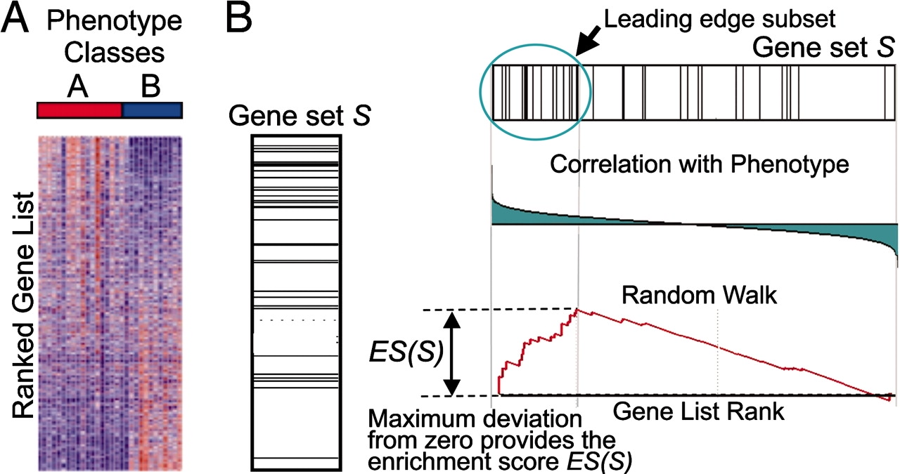
This image describes the theory of GSEA, with the 'gene set S' showing the metric used (in our case, ranked log2 fold changes) to determine enrichment of genes in the gene set. The left-most image is representing this metric used for the GSEA analysis. The log2 fold changes for each gene in the 'gene set S' is shown as a line in the middle image. The large positive log2 fold changes are at the top of the gene set image, while the largest negative log2 fold changes are at the bottom of the gene set image. In the right-most image, the gene set is turned horizontally, underneath which is an image depicting the calculations involved in determining enrichment, as described below.
Step 1: Calculation of enrichment score:
An enrichment score for a particular gene set is calculated by walking down the list of log2 fold changes and increasing the running-sum statistic every time a gene in the gene set is encountered and decreasing it when genes are not part of the gene set. The size of the increase/decrease is determined by magnitude of the log2 fold change. Larger (positive or negative) log2 fold changes will result in larger increases or decreases. The final enrichment score is where the running-sum statistic is the largest deviation from zero.
Step 2: Estimation of significance:
The significance of the enrichment score is determined using permutation testing, which performs rearrangements of the data points to determine the likelihood of generating an enrichment score as large as the enrichment score calculated from the observed data. Essentially, for this step, the first permutation would reorder the log2 fold changes and randomly assign them to different genes, reorder the gene ranks based on these new log2 fold changes, and recalculate the enrichment score. The second permutation would reorder the log2 fold changes again and recalculate the enrichment score again, and this would continue for the total number of permutations run. Therefore, the number of permutations run will increase the confidence in the signficance estimates.
Step 3: Adjust for multiple test correction
After all gene sets are tested, the enrichment scores are normalized for the size of the gene set, then the p-values are corrected for multiple testing.
The GSEA output will yield the core genes in the gene sets that most highly contribute to the enrichment score. The genes output are generally the genes at or before the running sum reaches its maximum value (e.g. the most influential genes driving the differences between conditions for that gene set).
Performing GSEA
To perform the GSEA using KEGG gene sets with clusterProfiler, we can use the gseKEGG() function:
## GSEA using gene sets from KEGG pathways
gseaKEGG <- gseKEGG(geneList = foldchanges, # ordered named vector of fold changes (Entrez IDs are the associated names)
              organism = "hsa", # supported organisms listed below
              pvalueCutoff = 0.05, # padj cutoff value
              verbose = FALSE)

## Extract the GSEA results
gseaKEGG_results <- gseaKEGG@result
head(gseaKEGG_results)
Other organisms for KEGG pathways
The organisms with KEGG pathway information are listed here.
How many pathways are enriched? Let's view the enriched pathways:
## Write GSEA results to file
View(gseaKEGG_results)

write.csv(gseaKEGG_results, "../Results/gseaCont-Vamp_kegg.csv", quote=F)
Warning
We will can all get different results for the GSEA because the permutations performed use random reordering. If we would like to use the same permutations every time we run a function (i.e. we would like the same results every time we run the function), then we could use the set.seed(123456) function prior to running. The input to set.seed() could be any number, but if you would want the same results, then you would need to use the same number as input.
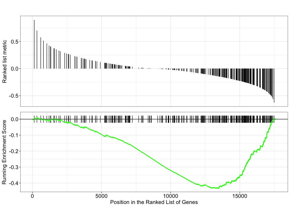
Explore the GSEA plot of enrichment of one of the pathways in the ranked list:
## Plot the GSEA plot for a single enriched pathway:
gseaplot(gseaKEGG, geneSetID = gseaKEGG_results$ID[1], title = gseaKEGG_results$Description[1])
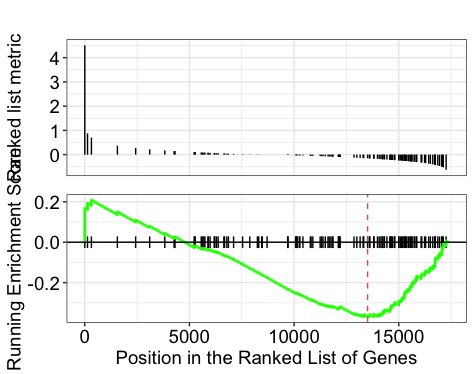
In this plot, the lines in plot represent the genes in the gene set, and where they occur among the log2 fold changes. The largest positive log2 fold changes are on the left-hand side of the plot, while the largest negative log2 fold changes are on the right. The top plot shows the magnitude of the log2 fold changes for each gene, while the bottom plot shows the running sum, with the enrichment score peaking at the red dotted line (which is among the negative log2 fold changes).
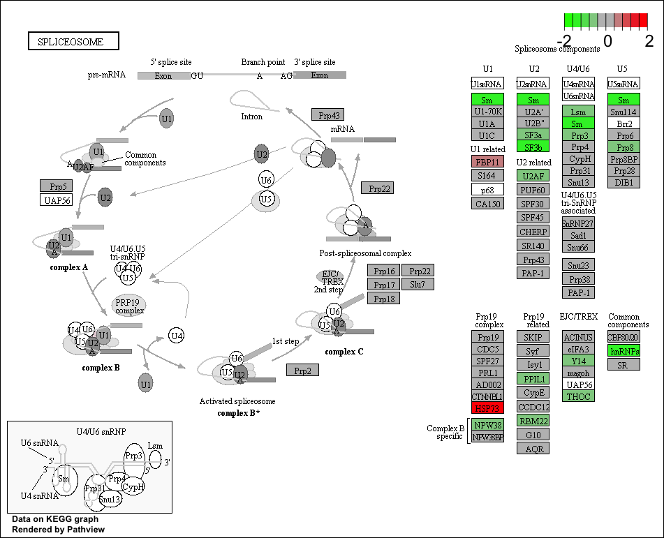
Use the Pathview R package to integrate the KEGG pathway data from clusterProfiler into pathway images:
## Output images for a single significant KEGG pathway
pathview(gene.data = foldchanges,
              pathway.id = gseaKEGG_results$ID[1],
              species = "hsa",
              limit = list(gene = 2, # value gives the max/min limit for foldchanges
              cpd = 1))
Printing out Pathview images for all significant pathways
Printing out Pathview images for all significant pathways can be easily performed as follows:
Instead of exploring enrichment of KEGG gene sets, we can also explore the enrichment of BP Gene Ontology terms using gene set enrichment analysis:
# GSEA using gene sets associated with BP Gene Ontology terms
gseaGO <- gseGO(geneList = foldchanges,
              OrgDb = org.Hs.eg.db,
              ont = 'BP',
              minGSSize = 20,
              pvalueCutoff = 0.05,
              verbose = FALSE)

gseaGO_results <- gseaGO@result
head(gseaGO_results)
There are other gene sets available for GSEA analysis in clusterProfiler (Disease Ontology, Reactome pathways, etc.). You can check out this link for more!
Exercise 1
Run a Disease Ontology (DO) GSE analysis using the gseDO() function. The arguments are very similar to the previous examples!
- Do you find anything interesting?
Solution to Exercise 1
We see now very similar results to our overrepresentation analysis. This is due to the fact that we have quite big lists of differentially expressed genes. GSEA analysis are most useful when your gene lists are low and normal overrepresentation analysis will perform very poorly.
Exercise 2
Run an GSE on the results of the DEA for Garlicum vs Vampirium samples. Remember to use the annotated results!
Solution to Exercise 2
We need to prepare our values for GSEA:
# Remove any NA values (reduces the data by quite a bit) and duplicates
res_entrez_Gar <- dplyr::filter(res_ids_Gar, entrez != "NA" & duplicated(entrez)==F)
Finally, extract and name the fold changes:
# Extract the foldchanges
foldchanges_Gar <- res_entrez_Gar$log2FoldChange

# Name each fold change with the corresponding Entrez ID
names(foldchanges_Gar) <- res_entrez_Gar$entrez
Next we need to order the fold changes in decreasing order. To do this we'll use the sort() function, which takes a vector as input. This is in contrast to Tidyverse's arrange(), which requires a data frame.
## Sort fold changes in decreasing order
foldchanges_Gar <- sort(foldchanges_Gar, decreasing = TRUE)

head(foldchanges_Gar)
Ne we can perform GSEA. This is an example for GO term analysis
Other Tools
Create your own Gene Set and run GSEA
It is possible to supply your own gene set GMT file, such as a GMT for MSigDB using special clusterProfiler functions as shown below:
# DO NOT RUN
BiocManager::install("GSEABase")
library(GSEABase)

# Load in GMT file of gene sets (we downloaded from the Broad Institute for MSigDB)

c2 <- read.gmt("/data/c2.cp.v6.0.entrez.gmt.txt")

msig <- GSEA(foldchanges, TERM2GENE=c2, verbose=FALSE)

msig_df <- data.frame(msig)
Pathway topology tools
Pathway topology analysis often takes into account gene interaction information along with the fold changes and adjusted p-values from differential expression analysis to identify dysregulated pathways. Depending on the tool, pathway topology tools explore how genes interact with each other (e.g. activation, inhibition, phosphorylation, ubiquitination, etc.) to determine the pathway-level statistics. Pathway topology-based methods utilize the number and type of interactions between gene product (our DE genes) and other gene products to infer gene function or pathway association.
For instance, the SPIA (Signaling Pathway Impact Analysis) tool can be used to integrate the lists of differentially expressed genes, their fold changes, and pathway topology to identify affected pathways.
Co-expression clustering
Co-expression clustering is often used to identify genes of novel pathways or networks by grouping genes together based on similar trends in expression. These tools are useful in identifying genes in a pathway, when their participation in a pathway and/or the pathway itself is unknown. These tools cluster genes with similar expression patterns to create 'modules' of co-expressed genes which often reflect functionally similar groups of genes. These 'modules' can then be compared across conditions or in a time-course experiment to identify any biologically relevant pathway or network information.
You can visualize co-expression clustering using heatmaps, which should be viewed as suggestive only; serious classification of genes needs better methods.
The way the tools perform clustering is by taking the entire expression matrix and computing pair-wise co-expression values. A network is then generated from which we explore the topology to make inferences on gene co-regulation. The WGCNA package (in R) is one example of a more sophisticated method for co-expression clustering.
Extra resources for functional analysis
- g:Profiler - http://biit.cs.ut.ee/gprofiler/index.cgi
- DAVID - http://david.abcc.ncifcrf.gov/tools.jsp
- clusterProfiler - http://bioconductor.org/packages/release/bioc/html/clusterProfiler.html
- GeneMANIA - http://www.genemania.org/
- GenePattern - http://www.broadinstitute.org/cancer/software/genepattern/ (need to register)
- WebGestalt - http://bioinfo.vanderbilt.edu/webgestalt/ (need to register)
- AmiGO - http://amigo.geneontology.org/amigo
- ReviGO (visualizing GO analysis, input is GO terms) - http://revigo.irb.hr/
- WGCNA - https://horvath.genetics.ucla.edu/html/CoexpressionNetwork/Rpackages/WGCNA/
- GSEA - http://software.broadinstitute.org/gsea/index.jsp
- SPIA - https://www.bioconductor.org/packages/release/bioc/html/SPIA.html
- GAGE/Pathview - http://www.bioconductor.org/packages/release/bioc/html/gage.html
This lesson was originally developed by members of the teaching team (Mary Piper, Radhika Khetani) at the Harvard Chan Bioinformatics Core (HBC).
Created: November 28, 2023