Practical material

Course Overview

⏰ Time Estimation: X minutes
💬 Learning Objectives:

1. Organize and structure your data and data analysis with Cookiecutter templates
2. Define metadata fields and collect metadata when creating a Cookiecutter folder
3. Establish naming conventions for your data
4. Create a catalog of your data
5. Use GitHub repositories of your data analysis and display them as GitHub Pages
6. Archive GitHub repositories on Zenodo

This practical version covers practical aspects of RDM applied to biodata. The exercises provided here aim to help you organize and structure your datasets and data analyses. You’ll learn how to manage your experimental metadata effectively and safely version control and archive your data analyses using GitHub repositories and Zenodo. Through these guided exercises and step-by-step instructions, we hope you will acquire essential skills for managing and sharing your research data efficiently, thereby enhancing the reproducibility and impact of your work.

Requirements

Ensure all necessary tools and software are installed before beginning the practical exercises:

• A GitHub account for hosting and collaborating on projects
• Git for version control of your projects
• A Zenodo account for archiving and sharing your research outputs
• Python
• pip for managing Python packages
• Cookicutter for creating folder structure templates (pip install cookiecutter)
• cruft to version control your templates (pip install cruft)

Two more tools will be required, choose the one you are familiar with or the first option:

• Option a. Install Quarto. We recommend Quarto as is easy to use and provides native support for notebooks (both R Markdown and Jupyter Notebooks). It requires no additional extensions or dependencies.
• Option b. Install MkDocs and MkDocs extensions using the command line. Additional extensions are optional but can be useful if you choose this approach.

pip install mkdocs # create webpages
pip install mkdocs-material # customize webpages
pip install mkdocs-video # add videos or embed videos from other sources
pip install mkdocs-minify-plugin # Minimize html code
pip install mkdocs-git-revision-date-localized-plugin # display last updated date 
pip install mkdocs-jupyter # include Jupyter notebooks
pip install mkdocs-bibtex # add references in your text (`.bib`)
pip install neoteroi-mkdocs # create author cards
pip install mkdocs-table-reader-plugin # embed tabular format files (`.tsv`)

1. Organize and structure your datasets and data analysis

Establishing a consistent file structure and naming conventions will help you efficiently manage your data. We will classify your data and data analyses into two distinct types of folders to ensure the data can be used and shared by many lab members while preventing modifications by any individual:

1. Data folders (assay or external databases and resources): They house the raw and processed datasets, alongside the pipeline/workflow used to generate the processed data, the provenance of the raw data, and quality control reports of the data. The data should be locked and set to read-only to prevent unintended modifications. This applies to experimental data generated in your lab as well as external resources. Provide an MD5 checksum file when you download them yourself to verify their integrity.
2. Project folders: They contain all the essential files for a specific research project. Projects may use data from various resources or experiments, or build upon previous results from other projects. The data should not be copied or duplicated, instead, it should be linked directly from the source.

Data and data analysis are kept separate because a project may utilize one or more datasets to address a scientific question. Data can be reused in multiple projects over time, combined with other datasets for comparison, or used to build larger datasets. Additionally, data may be utilized by different researchers to answer various research questions.

Hint

When organizing your data folders, separate assays from external resources and maintain a consistent structure. For example, organize genome references by species and further categorize them by versions. Make sure to include all relevant information, and refer to this lesson for additional tips on data organization.

This will help you to keep your data tidied up, especially if you are working in a big lab where assays may be used for different purposes and by different people!

Data folders

Whether your lab generates its own experimental data, receives it from collaborators, or works with previously published datasets, the data folder should follow a similar structure to the one presented here. Create a separate folder for each dataset, including raw files and processed files alongside the corresponding documentation and pipeline that generated the processed data. Raw files should remain untouched, and you should consider locking modifications to the final results once data preprocessing is complete. This precaution helps prevent unwanted changes to the data. Each subfolder should be named in a way that is distinct, easily readable and clear at a glance. Check this lesson for tips on naming conventions.

Hint

Use an acronym (1) that describes the type of NGS assay (RNAseq, ChIPseq, ATACseq) a keyword (2) that represents a unique element to that assay, and the date (3).

<Assay-ID>_<keyword>_YYYYMMDD

For example CHIP_Oct4_20230101 is a ChIPseq assay made on 1st January 2023 with the keyword Oct4, so it is easily identifiable by the eye.

Let’s explore a potential folder structure and the types of files you might encounter within it.

<data_type>_<keyword>_YYYYMMDD/
├── README.md 
├── CHECKSUMS
├── pipeline
    ├── pipeline.md
    ├── scripts/
├── processed
    ├── fastqc/
    ├── multiqc/
    ├── final_fastq/
└── raw
    ├── .fastq.gz 
    └── samplesheet.csv

• README.md: This file contains a detailed description of the dataset commonly in markdown format. It should include the provenance of the raw data (such as samples, laboratory protocols used, the aim of the project, folder structure, naming conventions, etc.).
• metadata.yml: This metadata file outlines different keys and essential information, usually presented in YAML format. For more details, refer to this lesson.
• pipeline.md: This file provides an overview of the pipeline used to process raw data, as well as the commands to run the pipeline. The pipeline itself and all the required scripts should be collected in the same directory.
• processed: This folder contains the results from the preprocessing pipeline. The content vary depending on the specific pipeline used (create additional subdirectories as needed).
• raw: This folder holds the raw data.
  • .fastq.gz: For example, in NGS assays, there should be ‘fastq’ files.
  • samplesheet.csv: This file holds essential metadata for the samples, including sample identification, experimental variables, batch information, and other metrics crucial for downstream analysis. It is important that this file is complete and current, as it is key to interpreting results. If you are considering running nf-core pipelines, this file will be required.

Project folders

On the other hand, we have another type of folder called Projects which refers to data analyses that are specific to particular tasks, such as those involved in preparing a potential article. In this folder, you will create a subfolder for each project that you or your lab is working on. Each Project subfolder should include project-specific information, data analysis pipelines, notebooks, and scripts used for that particular project. Additionally, you should include an environment file with all the required software and dependencies needed for the project, including their versions. This helps ensure that the analyses can be easily replicated and shared with others.

The Project folder should be named in a way that is unique, easy to read, distinguishable, and clear at a glance. For example, you might name it based on the main author’s initials, the dataset being analyzed, the project name, a unique descriptive element related to the project, or the part of the project you are responsible for, along with the date:

<project>_<keyword>_YYYYMMDD

Naming examples

• RNASeq_Mouse_Brain_20230512: a project RNA sequencing data from a mouse brain experiment, created on May 12, 2023
• EHR_COVID19_Study_20230115: a project around electronic health records data for a COVID-19 study, created on January 15, 2023.

Now, let’s explore an example of a folder structure and the types of files you might encounter within it.

<project>_<keyword>_YYYYMMDD
├── data
│  └── <ID>_<keyword>_YYYYMMDD <- symbolic link
├── documents
│  └── research_project_template.docx
├── metadata.yml
├── notebooks
│  └── 01_data_processing.rmd
│  └── 02_data_analysis.rmd
│  └── 03_data_visualization.rmd
├── README.md
├── reports
│  └── 01_data_processing.html
│  └── 02_data_analysis.html
│  ├── 03_data_visualization.html
│  │  └── figures
│  │  └── tables
├── requirements.txt // env.yaml
├── results
│  ├── figures
│  │  └── 02_data_analysis/
│  │    └── heatmap_sampleCor_20230102.png
│  ├── tables
│  │  └── 02_data_analysis/
│  │    └── DEA_treat-control_LFC1_p01.tsv
│  │    └── SumStats_sampleCor_20230102.tsv
├── pipeline
│  ├── rules // processes 
│  │  └── step1_data_processing.smk
│  └── pipeline.md
├── scratch
└── scripts

• data: This folder contains symlinks or shortcuts to the actual data files, ensuring that the original files remain unaltered.
• documents: This folder houses Word documents, slides, or PDFs associated with the project, including data and project explanations, research papers, and more. It also includes the Data Management Plan.
  • research_project_template.docx. If you download our template you will find a is a pre-filled Data Management Plan based on the Horizon Europe guidelines named ‘Non-sensitive_NGS_research_project_template.docx’.
• metadata.yml: metadata file describing various keys of the project or experiment (see this lesson).
• notebooks: This folder stores Jupyter, R Markdown, or Quarto notebooks containing the data analysis. Figures and tables used for the reports are organized under subfolders named after the notebook that created them for provenance purposes.
• README.md: A detailed project description in markdown or plain-text format.
• reports: Notebooks rendered as HTML, docx, or PDF files for sharing with colleagues or as formal data analysis reports.
  • figures: figures produced upon rendering notebooks. The figures will be saved under a subfolder named after the notebook that created them. This is for provenance purposes so we know which notebook created which figures.
• requirements.txt: This file lists the necessary software, libraries, and their versions required to reproduce the code. If you’re using conda environments, you will also find the env.yaml file here, which outlines the specific environment configuration.
• results: This folder contains analysis results, such as figures and tables. Organizing results by the pipeline, script, or notebook that generated them will make it easier to locate and interpret the data.
• pipeline: A folder containing pipeline scripts or workflows for processing and analyzing data.
• scratch: A folder designated for temporary files or workspace for experiments and development.
• scripts: Folder for helper scripts needed to run data analysis or reproduce the work.

Template engine

Creating a folder template is straightforward with cookiecutter a command-line tool that generates projects from templates (called cookiecutters). For example, it can help you set up a Python package project based on a Python package project template.

Cookiecutter templates

Here are some template that you can use to get started, adapt and modify them to your own needs:

• Python package project
• Sandbox test
• Data science
• NGS data

Create your own template from scratch.

Quick tutorial on cookiecutter

Building a Cookiecutter template from scratch requires defining a folder structure, crafting a cookiecutter.json file, and outlining placeholders (keywords) that will be substituted when generating a new project. Here’s a step-by-step guide on how to proceed:

Step 1: Create a Folder Template

First, begin by creating a folder structure that aligns with your desired template design. For instance, let’s set up a simple Python project template:

my_template/
|-- {{cookiecutter.project_name}}
|   |-- main.py
|-- tests
|   |-- test_{{cookiecutter.project_name}}.py
|-- README.md

In this example, {cookiecutter.project_name} is a placeholder that will be replaced with the actual project name when the template is used. This directory contains a python script (‘main.py’), a subdirectory (‘tests’) with a second python script named after the project (‘test_{{cookiecutter.project_name}}.py’) and a ‘README.md’ file.

Step 2: Create cookiecutter.json

In the root of your template folder, create a file named cookiecutter.json. This file will define the variables (keywords) that users will be prompted to fill in. For our Python project template, it might look like this:

{
  "project_name": "MyProject",
  "author_name": "Your Name",
  "description": "A short description of your project"
}

When users generate a project based on your template, they will be prompted with these questions. The provided values (“responses”) will be used to substitute the placeholders in your template files.

Beyond substituting placeholders in file and directory names, Cookiecutter can automatically populate text file contents with information. This feature is useful for offering default configurations or code file templates. Let’s enhance our earlier example by incorporating a placeholder within a text file:

First, modify the my_template/main.py file to include a placeholder inside its contents:

main.py

# main.py
def hello():
    print("Hello, {{cookiecutter.project_name}}!")

The ‘{{cookiecutter.project_name}}’ placeholder is now included within the main.py file. When you execute Cookiecutter, it will automatically replace the placeholders in both file and directory names and within text file contents.

After running Cookiecutter, your generated ‘main.py’ file could appear as follows:

# main.py, assuming "MyProject" was entered as the project_name
def hello():
    print("Hello, MyProject!") 

Step 3: Use Cookiecutter

Once your template is prepared, you can utilize Cookiecutter to create a project from it. Open a terminal and execute:

cookiecutter path/to/your/template

Cookiecutter will prompt you to provide values for project_name, author_name, and description. Once you input these values, Cookiecutter will replace the placeholders in your template files with the entered values.

Step 4: Review the Generated Project

After the generation process is complete, navigate to the directory where Cookiecutter created the new project. You will find a project structure with the placeholders replaced by the values you provided.

Exercise 1: Create your own template

Use Cookiecutter to create custom templates for your folders. You can do it from scratch (see Exercise 1, part B) or opt for one of our pre-made templates available as a Github repository (recommended for this workshop). Feel free to tailor the template to your specific requirements—you don’t have to follow our examples exactly.

Requirements

We assume you have already gone through the requirements at the beginning of the practical lesson. This includes installing the necessary tools and setting up accounts as needed.

Project

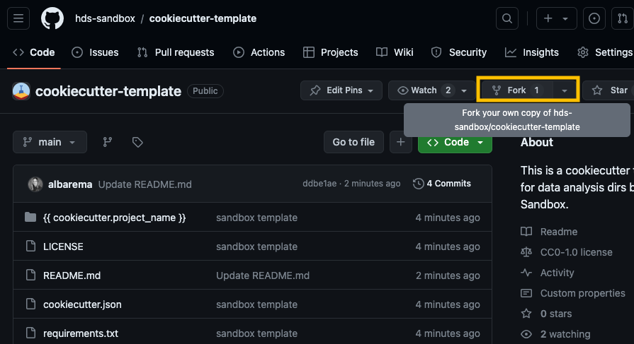
1. Go to our Cookicutter template and click on the Fork button at the top-right corner of the repository page to create a copy of the repository on your own GitHub account or organization.

2. Open a terminal on your computer, copy the URL of your fork and clone the repository to your local machine (the URL should look something like https://github.com/your_username/cookiecutter-template):

   git clone <your URL to the template>

   If you have a GitHub Desktop, click Add and select “Clone repository” from the options

3. Open the repository and navigate through the different directories

4. Modify the contents of the repository as needed to fit your project’s requirements. You can change files, add new ones. remove existing one or adjust the folder structure. For inspiration, review the data structure above under ‘Project folder’. For instance, this template is missing the ‘reports’ directory and add the ‘requirements.txt’ file. Consider creating it, along with a subdirectory named ‘reports/figures’.

   ├── results/
   │   ├── figures/
   ├── requirements.txt

   Here’s an example of how to do it:

   # Open your terminal and navigate to your template directory. Then: 
   cd \{\{\ cookiecutter.project_name\ \}\}/  
   mkdir reports 
   touch requirements.txt

5. Commit and push changes when you are done with your modifications

• Stage the changes with git add
• Commit the changes with a meaningful commit message git commit -m "update cookicutter template"
• Push the changes to your forked repository on Github git push origin main (or the appropriate branch name)

6. Test your template by using cookiecutter <URL to your GitHub repository "cookicutter-template">

   Fill up the variables and verify that the new structure (and folders) looks like you would expect. Have any new folders been added, or have some been removed?

Optional Exercise 1, part B

Create a template from scratch using this tutorial scratch, it can be as basic as this one below or ‘Data folder’:

my_template/
|-- {{cookiecutter.project_name}}
|   |-- main.py
|-- tests
|   |-- test_{{cookiecutter.project_name}}.py
|-- README.md

• Step 1: Create a directory for the template.
• Step 2: Write a cookiecutter.json file with variables such as project_name and author.
• Step 3: Set up the folder structure by creating subdirectories and files as needed.
• Step 4: Incorporate cookiecutter variables in the names of files.
• Step 5: Use cookiecutter variables within scripts, such as printing a message that includes the project name.

2. Data documentation

Data documentation involves organizing, describing, and providing context for datasets and projects. While metadata concentrates on the data itself, README files provide a broader perspective on the overall project or resource.

Metadata

metadata.yml

Choose the format that best suits the project’s needs. In this workshop, we will focus on YAMl as it is highly used for configuration files (e.g., in conda or pipelines).

File formats

• XML (eXtensible Markup Language): uses custom tags to describe data and allows for a hierarchical structure.
• JSON (JavaScript Object Notation): lightweight and human-readable format that is easy to parse and generate.
• CSV (Comma-Separated Values) or TSV (tabulate-separate values): simple and widely supported for representing tabular formats. Easy to manipulate using software or programming languages. It is often use for sample metadata.
• YAML (YAML Ain’t Markup Language): human-readable data serialization format, commonly used as project configuration files.

Others such as RDF or HDF5.

Link to the file format database.

Metadata in biological datasets refers to the information that describes the data and provides context for how the data was collected, processed, and analyzed. Metadata is crucial for understanding, interpreting, and using biological datasets effectively. It also ensures that datasets are reusable, reproducible and understandable by other researchers. Some of the components may differ depending on the type of project, but there are general concepts that will always be shared across different projects:

• Sample information and collection details
• Biological context (such experimental conditions if applicable)
• Data description
• Data processing steps applied to the raw data
• Annotation and Ontology terms
• File metadata (file type, file format, etc.)
• Ethical and Legal Compliance (ownership, access, provenance)

Metadata and controlled vocabularies

To maximize the usefulness of metadata, aim to use controlled vocabularies across all fields. Read more about data documentation and find ontology services examples in lesson 4. We encourage you to begin implementing them systematically on your own (under the “sources” section, you will find some helpful links to guide you putting them in practice).

If you work with NGS data, check out this recommendations and examples of metadata for samples, projects and datasets.

README file

README.md

Choose the format that best suits the project’s needs. In this workshop, we will focused on Markdown as it is the most used format due to its balance of simplicity and expressive formatting options.

File formats

• Markdown (.md): commonly used because is easy to read and write and is compatible across platforms (e.g., GitHub, GitLab). Supports formatting like headings, lists, links, images, and code blocks.
• Plain Text (.txt): Simple and straightforward format without any rich formatting and great for basic instructions. Lack the ability of structure content effectively.
• ReStructuredText (.rst): commonly used for python projects. Supports advanced formatting (takes, links, images and code blocks) .

Others such as HTML, YAML and Notebooks.

Link to the file format database

The README.md file is a markdown file that provides a comprehensive description of the data within a folder. Its rich text format (including bold, italic, links, etc.) allows you to explain the contents of the folder, as well as the reasons and methods behind its creation or collection. The content will vary depending on what it described (data or assays, project, software…).

Here is an example of a README file for a bioinformatics project:

README

# TITLE

Clear and descriptive.

# OVERVIEW

Introduction to the project including its aims, and its significance. Describe the main purpose and the biological questions being addressed.

Example text

This project aims to investigate gene expression patterns across various human tissues using Next Generation Sequencing (NGS) data. By analyzing the transcriptomes of different tissues, we seek to uncover tissue-specific gene expression profiles and identify potential markers associated with specific biological functions or diseases.

Understanding tissue-specific gene expression is crucial for deciphering the molecular basis of health and disease. Identifying genes that are uniquely expressed in certain tissues can provide insights into tissue function, development, and potential therapeutic targets. This project contributes to our broader understanding of human biology and has implications for personalized medicine and disease research.

# TABLE OF CONTENTS (optional but helpful for others to navigate to different sections)

# INSTALLATION AND SETUP

List all prerequisites, software, dependencies, and system requirements needed for others to reproduce the project. If available, you may link to a Docker image, Conda YAML file, or requirements.txt file.

# USAGE

Include command-line examples for various functionalities or steps and path for running a pipeline, if applicable.

# DATASETS

Describe the data,, including its sources, format, and how to access it. If the data has undergone preprocessing, provide a description of the processes applied or the pipeline used.

Example text

We have used internal datasets with IDs: RNA_humanSkin_20201030, RNA_humanBrain_20210102, RNA_humanLung_20220304.

In addition, we utilized publicly available NGS datasets from the GTEx (Genotype-Tissue Expression) project, which provides comprehensive RNA-seq data across multiple human tissues. These datasets offer a wealth of information on gene expression levels and isoform variations across diverse tissues, making them ideal for our analysis.

# RESULTS

Summarize the results and key findings or outputs.

Example text

Our analysis revealed distinct gene expression patterns among different human tissues. We identified tissue-specific genes enriched in brain tissues, highlighting their potential roles in neurodevelopment and function. Additionally, we found a set of genes that exhibit consistent expression across a range of tissues, suggesting their fundamental importance in basic cellular processes.

Furthermore, our differential expression analysis unveiled significant changes in gene expression between healthy and diseased tissues, shedding light on potential molecular factors underlying various diseases. Overall, this project underscores the power of NGS data in unraveling intricate gene expression networks and their implications for human health.

# CONTRIBUTIONS AND CONTACT INFO

# LICENSE

Exercise 2: modify the metadata.yml file in your Cookiecutter template

It is time now to customize your Cookiecutter templates and modify the metadata.yml files so that they fit your needs!

0. Consider changing variables (add/remove) in the metadata.yml file from the cookicutter template.

1. Modify the cookiecutter.json file. You could add new variables or change the default key and/or values:

   cookiecutter.json

   {
   "project_name": "myProject",
   "project_slug": "{{ cookiecutter.project_name.lower().replace(' ', '_').replace('-', '_') }}",
   "authors": "myName",
   "start_date": "{% now 'utc', '%Y%m%d' %}",
   "short_desc": "",
   "version": "0.1.0"
   }

   The metadata file will be filled accordingly.

2. Optional: You can customize or remove this prompt message entirely, allowing you to tailor the text to your preferences for a unique experience each time you use the template.

   cookiecutter.json

   "__prompts__": {
       "project_name": "Project directory name [Example: project_short_description_202X]",
       "author": "Author of the project",
       "date": "Date of project creation, default is today's date",
       "short_description": "Provide a detailed description of the project (context/content)"
   },

3. Modify the metadata.yml file so that it includes the metadata recorded by the cookiecutter.json file. Hint below:

   metadata.yml

   project: {{ cookiecutter.project_name }}
   author: {{ cookiecutter.author }}
   date: {{ cookiecutter.date }}
   description: {{ cookiecutter.short_description }}

4. Modify the README.md file so that it includes the short description recorded by the cookiecutter.json file and the metadata at the top of the markdown file (top between lines of dashed).

   README.md

   ---
   title: {{ cookiecutter.project_name }}
   date: "{{ cookiecutter.date }}"
   author: {{ cookiecutter.author }}
   version: {{ cookiecutter.version }}
   ---
   
   Project description
   ----
   
   {{ cookiecutter.short_description }}

5. Commit and push changes when you are done with your modifications

• Stage the changes with git add
• Commit the changes with a meaningful commit message git commit -m "update cookicutter template"
• Push the changes to your forked repository on Github git push origin main (or the appropriate branch name)

6. Test your template by using cookiecutter <URL to your GitHub repository "cookicutter-template">

   Fill up the variables and verify that the modified information looks like you would expect.

3. Naming conventions

As discussed in lesson 3, consistent naming conventions are key for interpreting, comparing, and reproducing findings in scientific research. Standardized naming helps organize and retrieve data or results, allowing researchers to locate and compare similar types of data within or across large datasets.

Exercise 3: Define your file name conventions

Avoid long and complicated names and ensure your file names are both informative and easy to manage:

1. For saving a new plot, a heatmap representing sample correlations
2. When naming the file for the document containing the Research Data Management Course Objectives (Version 2, 2nd May 2024) from the University of Copenhagen
3. Consider the most common file types you work with, such as visualizations, figures, tables, etc., and create logical and clear file names

Hint

1. heatmap_sampleCor_20240101.png
2. KU_RDM-objectives_20240502_v02.doc or KU_RDMObj_20240502_v02.doc

4. Create a catalog of your data folder

The next step is to collect all the datasets that you have created in the manner explained above. Since your folders all should contain the metadata.yml file in the same place with the same metadata, it should be very easy to iteratively go through all the folders and merge all the metadata.yml files into a one single table. he table can be easily viewed in your terminal or even with Microsoft Excel.

Exercise 4: create a metadata.tsv catalog

We will make a small script in R (or you can make one with Python) that recursively goes through all the folders inside an input path (like your Assays folder), fetches all the metadata.yml files, merges them and writes a TSV file as an output.

1. Create a folder called dataset and change directory cd dataset
2. Fork this repository: a Cookiecutter template designed for NGS datasets.While you are welcome to create your own template from scratch, we recommend using this one to save time.
3. Run the cookiecutter cc-data-template command at least twice to create multiple datasets or projects. Use different values each time to simulate various scenarios (do this in the dataset directory that you have previously created).
4. Execute the script below using R (or create your own script in Python). Adjust the folder_path variable so that it matches the path to the Assays folder. The resulting table will be saved in the same folder_path.
5. Open your database_YYYYMMDD.tsv table in a text editor from the command-line, or view it in Excel for better visualization.

• Solution A. From a TSV

Hint

# R version 4.3.2
# RScript to read all yaml files in directory and save the metadata into a dataframe
quiet <- function(package_name) {
  # Suppress warnings and messages while checking and installing the package
  suppressMessages(suppressWarnings({
    # Check if the package is available and load it
    if (!requireNamespace(package_name, quietly = TRUE)) {
      install.packages(package_name)
    }
    # Load the package
    library(package_name, character.only = TRUE)
  }))
}

# Check and install necessary libraries
quiet("yaml")
quiet("dplyr")
quiet("lubridate")


read_yaml <- function(file_path) {
  # Read the YAML file and convert it to a data frame
  df <- yaml::yaml.load_file(file_path) %>% as.data.frame(stringsAsFactors = FALSE)
  
  # Return the data frame
  return(df)
}

# Function to recursively fetch metadata.yml files
get_metadata <- function(folder_path) {
  file_list <- list.files(path = folder_path, pattern = "metadata\\.yml$", recursive = TRUE, full.names = TRUE)

  metadata_list <- lapply(file_list, read_yaml)
  
  # Combine the list of data frames into a single data frame using dplyr::bind_rows()
  combined_metadata <- bind_rows(metadata_list)

  return(combined_metadata)
}

# Specify the folder path
folder_path <- "./" #/path/to/your/folder

# Fetch metadata from the specified folder
df <- get_metadata(folder_path)

# Save the data frame as a TSV file
output_file <- paste0("database_", format(Sys.Date(), "%Y%m%d"), ".tsv")
write.table(df, file = output_file, sep = "\t", quote = FALSE, row.names = FALSE)

# Print confirmation message
cat("Database saved as", output_file, "\n")

Exercise 4, option B: create a SQLite database

Alternatively, create a SQLite database from a metadata. If you opt for this option in the exercise, you must still complete the first three steps outlined above. Read more from the RSQLite documentation.

• Solution B. SQLite database

Hint

print("Assuming the libraries from Exercise 4 are already loaded and a dataframe has been generated from the YAML files...")

# check_and_install() form Exercise 4, and load the other packages. 
quiet("DBI")
quiet("RSQLite")

# Initialize a temporary in memory database and copy the data.frame into it

db_file_path <- paste0("database_", format(Sys.Date(), "%Y%m%d"), ".sqlite")
con <- dbConnect(RSQLite::SQLite(), db_file_path)

dbWriteTable(con, "metadata", df,  overwrite=TRUE) #row.names = FALSE,append =

# Print confirmation message
cat("Database saved as", db_file_path, "\n")

# Close the database connection
dbDisconnect(con)

Shiny apps

To get the most out of your metadata file and the ones from other colleagues, you can combine them and explore them by creating an interactive catalog browser. You can create interactive web apps straight from R or Python. Whether you have generated a tabulated-file or a sqlite database, browse through the metadata using Shiny. Shiny apps are perfect for researchers because they enable you to create interactive visualizations and dashboards with dynamic data inputs and outputs without needing extensive web development knowledge. Shiny provides a variety of user interface components such as forms, tables, graphs, and maps to help you organize and present your data effectively. It also allows you to filter, sort, and segment data for deeper insights.

Tip

• For R Enthusiasts

Explore demos from the R Shiny community to kickstart your projects or for inspiration.

• For python Enthusiasts

Shiny for Python provides live, interactive code throughout its entire tutorial. Additionally, it offers a great tool called Playground, where you can code and test your own app to explore how different features render.

Exercise 5: Skill Booster, build an interactive catalog browser

Build an interactive web app straight from R or Python. Below, you will find an example of an R shiny app. In either case, you will need to define a user interface (UI) and a server function. The UI specifies the layout and appearance of the app, including input controls and output displays. The server function contains the app’s logic, handling data manipulation, and responding to user interactions. Once you set up the UI and server, you can launch the app!

Here’s the UI and server function structure for an R Shiny app:

# Don't forget to load shiny and DT libraries!

# Specify the layout
ui <- fluidPage(
    titlePanel(...)
    # Define the appearance of the app
    sidebarLayout(
        sidebarPanel(...)
        mainPanel(...)
    )
)

server <- function(input, output, session) {
    # Define a reactive expression for data based on user inputs
    data <- reactive({
        req(input$dataInput)  # Ensure data input is available
        # Load or manipulate data here
    })

    # Define an output table based on data
    output$dataTable <- renderTable({
        data()  # Render the data as a table
    })

    # Observe a button click event and perform an action
    observeEvent(input$actionButton, {
        # Perform an action when the button is clicked
    })

    # Define cleanup tasks when the app stops
    onStop(function() {
        # Close connections or save state if necessary
    })
}
# Run the app
shinyApp(ui, server)

If you need more assistance, take a look at the code below (Hint).

Hint

# R version 4.3.2
print("Assuming the libraries from Exercise 4 are already loaded and a dataframe has been generated from the YAML files...")

# check_and_install() form Exercise 4. 
quiet("shiny")
quiet("DT")

# UI
ui <- fluidPage(
  titlePanel("TSV File Viewer"),
  
  sidebarLayout(
    sidebarPanel(
      fileInput("file", "Choose a TSV file", accept = c(".tsv")),
      selectInput("filter_column", "Filter by Column:", choices = c("n_samples", "technology"), selected = "technology"),
      textInput("filter_value", "Filter Value:", value = ""),
      # if only numbers, numericInput()
      radioButtons("sort_order", "Sort Order:", choices = c("Ascending", "Descending"), selected = "Ascending")
    ),
    
    mainPanel(
      DTOutput("table")
    )
  )
)

# Server
server <- function(input, output) {
  
  data <- reactive({
    req(input$file)
    df <- read.delim(input$file$datapath, sep = "\t")
    print(str(df))

    # Filter the DataFrame based on user input
    if (input$filter_column != "" && input$filter_value != "") {
      # Check if the column is numeric, and filter for value
      if (is.numeric(df[[input$filter_column]])) {
        df <- df[df[[input$filter_column]] >= as.numeric(input$filter_value), ]
      }
      # Check if the column is a string
      else if (is.character(df[[input$filter_column]])) {
        df <- df[df[[input$filter_column]] == input$filter_value, ]
      }
    }
    
    # Sort the DataFrame based on user input
    sort_order <- if (input$sort_order == "Ascending") TRUE else FALSE
    df <- df[order(df[[input$filter_column]], decreasing = !sort_order), ]
    df
  })
  
  output$table <- renderDT({
    datatable(data())
  })
}

# Run the app
shinyApp(ui, server)

In the optional exercise below, you’ll find a code example for using an SQLite database as input instead of a tabulated file.

Exercise (optional)

Once you’ve finished the previous exercise, consider implementing these additional ideas to maximize the utility of your catalog browser.

• Use SQLite databases as input
• Add a functionality to only select certain columns uiOutput("column_select")
• Filter columns by value using column_filter_select()
• Add multiple tabs using tabsetPanel()
• Add buttons to order numeric columns ascending or descending using radioButtons()
• Use SQL aggregation functions (e.g., SUM, COUNT, AVG) to perform custom data summaries and calculations.
• Add a tab tabPanel() to create a project directory interactively (and fill up the metadata fields), tips: dir.create(), data.frame(), write.table()
• Modify existing entries
• Visualize results using Cirrocumulus, an interactive visualization tool for large-scale single-cell genomics data.

If you need some assistance, take a look at the code below (Hint).

Hint

Explore an example with advanced features such as a two-tab layout, filtering by numeric values and matching strings, and a color-customized dashboard here.

5. Version control using Git and GitHub

Version control involves systematically tracking changes to a project over time, offering a structured way to document revisions and understand the progression of your work. In research data management and data analytics, it plays a critical role and provides numerous benefits.

Git is a distributed version control system that helps developers and researchers efficiently manage project history, collaborate seamlessly, and maintain data integrity. On the other hand, GitHub is a web-based platform that builds on Git’s functionality by providing a centralized, collaborative hub for hosting Git repositories. It offers several key functionalities, such as tracking issues, security features to safeguard your repos, and GitHub Pages that allow you to create websites to showcase your projects.

Create a GitHub organization for your lab or department

GitHub users can create organizations, allowing groups to collaborate or create repositories under the same organization umbrella. You can create an educational organization on Github for free, by setting up a Github account for your lab.

Follow these instructions to create a GitHub organization.

Once you’ve established your GitHub organization, be sure to create your repositories within the organization’s space rather than under your personal user account. This keeps your projects centralized and accessible to the entire group. Best practices for managing an organization on GitHub include setting clear access permissions, regularly reviewing roles and memberships, and organizing repositories effectively to keep your projects structured and easy to navigate.

Setting up a GitHub repository for your project folder

Version controlling your data analysis folders becomes straightforward once you’ve established your Cookiecutter templates. After you’ve created several folder structures and metadata using your Cookiecutter template, you can manage version control by either converting those folders into Git repositories or copying a folder into an existing Git repository. Both approaches are explained in Lesson 5.

Exercise 6: initialize a repository from an existing folder:

1. Initialize the repository: Begin by running the command git init in your project directory. This command sets up a new Git repository in the current directory and is executed only once, even for collaborative projects. See (git init) for more details.
2. Create a remote repository: Once the local repository is initialized, create an empty new repository on GitHub (website or Github Desktop).
3. Connect the remote repository: Add the GitHub repository URL to your local repository using the command git remote add origin <URL>. This associates the remote repository with the name “origin.”
4. Commit changes: If you have files you want to add to your repository, stage them using git add ., then create a commit to save a snapshot of your changes with git commit -m "add local folder".
5. Push to GitHub: To synchronize your local repository with the remote repository and establish a tracking relationship, push your commits to the GitHub repository using git push -u origin main.

Tips to write good commit messages

If you would like to know more about Git commits and the best way to make clear Git messages, check out this post!

GitHub Pages

After creating your repository and hosting it on GitHub, you can now add your data analysis reports—such as Jupyter Notebooks, R Markdown files, or HTML reports—to a GitHub Page website. Setting up a GitHub Page is straightforward, and we recommend following GitHub’s helpful tutorial. However, we will go through the key steps in the exercise below. There are several ways to create your web pages, but we suggest using Quarto as a framework to build a sleek, professional-looking website with ease. The folder templates from the previous exercise already contain the necessary elements to launch a webpage. Familiarizing yourself with the basics of Quarto will help you design a webpage that suits your preferences. Other common options include MkDocs. If you want to use MkDocs instead, click here and follow the instructions.

Tip

Here are some useful links to get started with Github Pages:

• Github Pages
• Quarto Github Pages

Exercise 7: Create a Github Page using Quarto

1. Head over to GitHub and create a new public repository named username.github.io, where username is your username (or organization name) on GitHub. If the first part of the repository doesn’t exactly match your username, it won’t work, so make sure to get it right.

2. Go to the folder where you want to store your project, and clone the new repository: git clone https://github.com/username/username.github.io (or use Github Desktop)

3. Create a new file named _quarto.yml

   _quarto.yml

   project:
       type: website

4. Open the terminal ```{.bash filename=“Terminal”} # Add a .nojekyll file to the root of the repository not to do additional processing of your published site touch .nojekyll #copy NUL .nojekyll for windows

   # Render and push it to Github quarto render git commit -m “Publish site to docs/” git push ```

5. If you do not have a gh-pages, you can create one as follows

   Terminal

   git checkout --orphan gh-pages
   git reset --hard # make sure all changes are committed before running this!
   git commit --allow-empty -m "Initialising gh-pages branch"
   git push origin gh-pages

6. Before attempting to publish you should ensure that the Source branch for your repository is gh-pages and that the site directory is set to the repository root (/)

   

7. It is important to not check your _site directory into version control, add the output directory of your project to .gitignore

   .gitignore

   /.quarto/
   /_site/

8. Now is time to publish your website

   .Terminal

   quarto publish gh-pages

9. Once you’ve completed a local publish, add a publish.yml GitHub Action to your project by creating this YAML file and saving it to .github/workflows/publish.yml. Read how to do it here

6. Archive GitHub repositories on Zenodo

Archives are specialized digital platforms that provide secure storage, curation, and dissemination of scientific data. They play a crucial role in the research community by acting as trusted repositories for preserving valuable datasets. With standardized formats and thorough curation processes, they ensure the long-term accessibility and citability of research findings. Researchers globally rely on these repositories to share, discover, and validate scientific information, promoting transparency, collaboration, and knowledge growth across various fields.

In the next practical exercise, you will archive your Project folder, which contains data analyses (software, code and pipelines), in a repository such as Zenodo. This can be done by linking your Zenodo account to your GitHub account.

Archiving data…

Data should be deposited in a domain-specific archive. If you want to know more about these archives, check out this lesson.

Zenodo

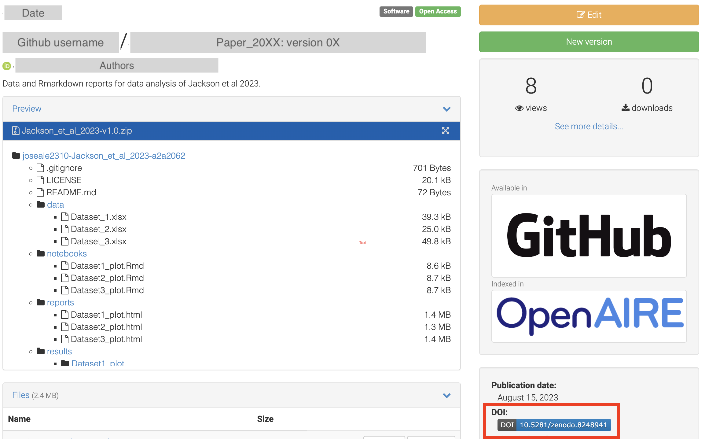
Zenodo is an open-access digital repository that supports the archiving of scientific research outputs, including datasets, papers, software, and multimedia files. Affiliated with CERN and backed by the European Commission, Zenodo promotes transparency, collaboration, and the advancement of knowledge globally. Researchers can easily upload, share, and preserve their data on its user-friendly platform. Each deposit receives a unique DOI for citability and long-term accessibility. Zenodo also offers robust metadata options and allows linking your GitHub account to archive a specific release of your GitHub repository directly to Zenodo. This integration streamlines the process of preserving a snapshot of your project’s progress.

Exercise 6: Archive a Project GitHub repo in Zenodo

1. In order to archive your GitHub repos in Zenodo, link your Zenodo and GitHub accounts
2. Once your accounts are linked, go to your Zenodo GitHub account settings and turn on the GitHub repository you want to archive.
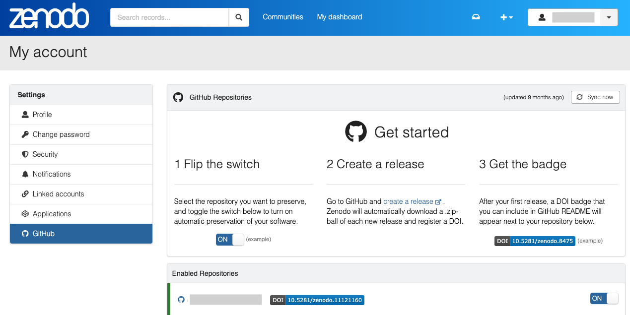
3. Creating a Zenodo archive is now as simple as making a release in your GitHub repository. Remember to create a proper tag and specify the version.
   NOTE: If you make a release before enabling the GitHub repository in Zenodo, it will not appear in Zenodo!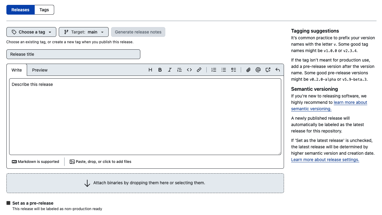
4. Zenodo will automatically detect the release and it should appear on your Zenodo upload page: My dashboard > Uploads.
5. This archive is assigned a unique Digital Object Identifier (DOI), making it a citable reference for your work.

Before submitting your work in a journal, make sure to link your data analysis repository to Zenodo, get a DOI, and cite it in your manuscript!

Wrap up

In this small workshop, we have learned how to improve the FAIRability of your data, as well as organize and structure it in a way that will be much more useful in the future. These advantages do not serve yourself only, but your teammates, group leader, and the general scientific population! We hope that you found this workshop useful. If you would like to leave us some comments or suggestions, feel free to contact us.

Copyright

CC-BY-SA 4.0 license