suppressMessages(
suppressWarnings({
library(VennDiagram)
library(dplyr)
library(tibble)
library(formattable)
library(mixOmics)
library(pheatmap)
library(edgeR)
}))
Tutorial description
This tutorial will cover the steps for performing Differential Gene Expression on the RNA-seq data obtained from the alignment done on the first notebook. At the end of this tutorial you will be able to use R and edgeR to
- Perform preliminary analyses of the RNA-seq results
- Find differentially expressed genes between two conditions using
edgeR - Create your own contrasts for a specific differential expression test
- Do various useful plots to show your results
edgeR is a package to test for differentially expressed genes between our Control and Treatment Samples. You can read more about the edgeR package and its functionalities here. This exercise largely follows their user manual.
Load the necessary R libraries
EdgeR - Data filtering and Normalization
In the following steps we load the aligned data, then filter and normalize it. Some of the genes have no transcripts – or very few of them – across all samples, which motivates why we want to clean up the data.
File processing
The data for this exercise comes from the 12 tabular files with Reads per Gene counts generated by STAR Mapping in the raw-data alignment part of this course. We want to create a table where each column is a sample, and the content of the table are the read counts from STAR. We must merge the 12 files with Reads per Gene information into a single file.
You need to have previously executed the alignment notebook to be able to load the data. The commands below will find the text files whose names end with ReadsPerGene.out.tab, and will read and concatenate them into a unique table.
samples <- sort(system("find results/STAR_output/*_align_contigs_1_2 -name \"*ReadsPerGene.out.tab\"", intern=TRUE))
print(samples)
Read_counts <- do.call(cbind, lapply(samples, function(x) read.delim(file=x, header = FALSE)))
[1] "results/STAR_output/S10_align_contigs_1_2/S10_1_1ReadsPerGene.out.tab"
[2] "results/STAR_output/S10_align_contigs_1_2/S10_1_2ReadsPerGene.out.tab"
[3] "results/STAR_output/S10_align_contigs_1_2/S10_1_3ReadsPerGene.out.tab"
[4] "results/STAR_output/S10_align_contigs_1_2/S10_2_1ReadsPerGene.out.tab"
[5] "results/STAR_output/S10_align_contigs_1_2/S10_2_2ReadsPerGene.out.tab"
[6] "results/STAR_output/S10_align_contigs_1_2/S10_2_3ReadsPerGene.out.tab"
[7] "results/STAR_output/TI_align_contigs_1_2/TI_1_1ReadsPerGene.out.tab"
[8] "results/STAR_output/TI_align_contigs_1_2/TI_1_2ReadsPerGene.out.tab"
[9] "results/STAR_output/TI_align_contigs_1_2/TI_1_3ReadsPerGene.out.tab"
[10] "results/STAR_output/TI_align_contigs_1_2/TI_2_1ReadsPerGene.out.tab"
[11] "results/STAR_output/TI_align_contigs_1_2/TI_2_2ReadsPerGene.out.tab"
[12] "results/STAR_output/TI_align_contigs_1_2/TI_2_3ReadsPerGene.out.tab" The data frame has genes as rows and samples as columns and stores the gene expression counts (value representing the total number of sequence reads that originated from a particular gene in a sample) for each of the 12 samples. This data frame should have 12 columns and 366 rows.
A brief peep into the table:
Read_counts| V1 | V2 | V3 | V4 | V1.1 | V2.1 | V3.1 | V4.1 | V1.2 | V2.2 | ⋯ | V3 | V4 | V1 | V2 | V3.1 | V4.1 | V1.1 | V2.1 | V3.2 | V4.2 |
|---|---|---|---|---|---|---|---|---|---|---|---|---|---|---|---|---|---|---|---|---|
| <chr> | <int> | <int> | <int> | <chr> | <int> | <int> | <int> | <chr> | <int> | ⋯ | <int> | <int> | <chr> | <int> | <int> | <int> | <chr> | <int> | <int> | <int> |
| N_unmapped | 23 | 23 | 23 | N_unmapped | 26 | 26 | 26 | N_unmapped | 23 | ⋯ | 76 | 76 | N_unmapped | 66 | 66 | 66 | N_unmapped | 81 | 81 | 81 |
| N_multimapping | 7008 | 7008 | 7008 | N_multimapping | 10085 | 10085 | 10085 | N_multimapping | 10542 | ⋯ | 10065 | 10065 | N_multimapping | 7544 | 7544 | 7544 | N_multimapping | 9130 | 9130 | 9130 |
| N_noFeature | 3504 | 25247 | 25511 | N_noFeature | 4326 | 33506 | 34092 | N_noFeature | 4507 | ⋯ | 30019 | 31205 | N_noFeature | 1994 | 22035 | 21926 | N_noFeature | 2157 | 24430 | 24959 |
| N_ambiguous | 254 | 74 | 62 | N_ambiguous | 261 | 70 | 73 | N_ambiguous | 333 | ⋯ | 40 | 35 | N_ambiguous | 255 | 34 | 30 | N_ambiguous | 311 | 26 | 41 |
| g175 | 143 | 75 | 72 | g175 | 226 | 115 | 117 | g175 | 227 | ⋯ | 125 | 107 | g175 | 206 | 116 | 107 | g175 | 165 | 77 | 96 |
| g176 | 17 | 9 | 12 | g176 | 12 | 12 | 6 | g176 | 15 | ⋯ | 10 | 7 | g176 | 11 | 14 | 14 | g176 | 23 | 19 | 12 |
| g177 | 0 | 0 | 0 | g177 | 0 | 0 | 0 | g177 | 0 | ⋯ | 0 | 0 | g177 | 0 | 0 | 0 | g177 | 0 | 0 | 0 |
| g178 | 0 | 0 | 0 | g178 | 0 | 0 | 0 | g178 | 0 | ⋯ | 0 | 2 | g178 | 1 | 0 | 1 | g178 | 2 | 0 | 2 |
| g179 | 0 | 0 | 0 | g179 | 0 | 0 | 0 | g179 | 0 | ⋯ | 0 | 0 | g179 | 0 | 0 | 0 | g179 | 0 | 0 | 0 |
| g180 | 2773 | 1401 | 1372 | g180 | 5223 | 2635 | 2588 | g180 | 4350 | ⋯ | 1341 | 1334 | g180 | 1023 | 518 | 505 | g180 | 2565 | 1304 | 1261 |
| g181 | 473 | 228 | 245 | g181 | 679 | 341 | 338 | g181 | 583 | ⋯ | 349 | 301 | g181 | 459 | 221 | 238 | g181 | 410 | 213 | 197 |
| g182 | 19 | 12 | 7 | g182 | 15 | 11 | 4 | g182 | 20 | ⋯ | 4 | 2 | g182 | 5 | 3 | 2 | g182 | 4 | 1 | 3 |
| g183 | 0 | 0 | 0 | g183 | 0 | 0 | 0 | g183 | 0 | ⋯ | 0 | 0 | g183 | 0 | 0 | 0 | g183 | 0 | 0 | 0 |
| g184 | 30 | 13 | 17 | g184 | 22 | 15 | 7 | g184 | 50 | ⋯ | 64 | 43 | g184 | 69 | 39 | 30 | g184 | 89 | 50 | 39 |
| g185 | 0 | 0 | 0 | g185 | 2 | 0 | 2 | g185 | 0 | ⋯ | 0 | 0 | g185 | 0 | 0 | 0 | g185 | 1 | 0 | 1 |
| g186 | 1 | 1 | 0 | g186 | 0 | 0 | 0 | g186 | 0 | ⋯ | 0 | 0 | g186 | 0 | 0 | 0 | g186 | 0 | 0 | 0 |
| g187 | 1 | 0 | 1 | g187 | 1 | 1 | 0 | g187 | 2 | ⋯ | 12 | 16 | g187 | 32 | 17 | 15 | g187 | 29 | 17 | 12 |
| g188 | 316 | 159 | 157 | g188 | 285 | 142 | 143 | g188 | 417 | ⋯ | 213 | 189 | g188 | 809 | 402 | 407 | g188 | 547 | 277 | 270 |
| g189 | 0 | 0 | 0 | g189 | 0 | 0 | 0 | g189 | 0 | ⋯ | 0 | 0 | g189 | 0 | 0 | 0 | g189 | 0 | 0 | 0 |
| g190 | 14 | 9 | 5 | g190 | 18 | 10 | 8 | g190 | 29 | ⋯ | 4 | 16 | g190 | 7 | 3 | 4 | g190 | 6 | 4 | 2 |
| g191 | 2 | 2 | 0 | g191 | 2 | 2 | 0 | g191 | 1 | ⋯ | 0 | 0 | g191 | 0 | 0 | 0 | g191 | 0 | 0 | 0 |
| g192 | 1 | 1 | 0 | g192 | 1 | 0 | 1 | g192 | 1 | ⋯ | 2 | 1 | g192 | 8 | 4 | 4 | g192 | 2 | 0 | 2 |
| g193 | 208 | 114 | 94 | g193 | 231 | 120 | 111 | g193 | 301 | ⋯ | 74 | 54 | g193 | 160 | 84 | 76 | g193 | 91 | 49 | 42 |
| g194 | 40 | 19 | 21 | g194 | 41 | 25 | 16 | g194 | 37 | ⋯ | 4 | 4 | g194 | 105 | 47 | 58 | g194 | 25 | 13 | 12 |
| g195 | 54 | 22 | 32 | g195 | 85 | 46 | 39 | g195 | 85 | ⋯ | 33 | 34 | g195 | 68 | 34 | 34 | g195 | 56 | 26 | 30 |
| g196 | 77 | 50 | 27 | g196 | 120 | 66 | 54 | g196 | 118 | ⋯ | 23 | 19 | g196 | 20 | 7 | 13 | g196 | 34 | 16 | 18 |
| g197 | 1 | 1 | 0 | g197 | 6 | 4 | 2 | g197 | 5 | ⋯ | 17 | 15 | g197 | 16 | 7 | 9 | g197 | 17 | 9 | 8 |
| g198 | 14 | 10 | 4 | g198 | 27 | 15 | 12 | g198 | 10 | ⋯ | 2 | 0 | g198 | 2 | 2 | 0 | g198 | 0 | 0 | 0 |
| g199 | 0 | 0 | 0 | g199 | 0 | 0 | 0 | g199 | 0 | ⋯ | 0 | 0 | g199 | 1 | 0 | 1 | g199 | 0 | 0 | 0 |
| g200 | 57 | 28 | 29 | g200 | 80 | 42 | 38 | g200 | 94 | ⋯ | 2 | 3 | g200 | 47 | 21 | 26 | g200 | 5 | 1 | 4 |
| ⋮ | ⋮ | ⋮ | ⋮ | ⋮ | ⋮ | ⋮ | ⋮ | ⋮ | ⋮ | ⋱ | ⋮ | ⋮ | ⋮ | ⋮ | ⋮ | ⋮ | ⋮ | ⋮ | ⋮ | ⋮ |
| g145 | 0 | 0 | 0 | g145 | 0 | 0 | 0 | g145 | 0 | ⋯ | 0 | 0 | g145 | 0 | 0 | 0 | g145 | 0 | 0 | 0 |
| g146 | 293 | 158 | 135 | g146 | 330 | 173 | 157 | g146 | 350 | ⋯ | 216 | 215 | g146 | 151 | 90 | 61 | g146 | 226 | 122 | 104 |
| g147 | 6 | 2 | 4 | g147 | 3 | 2 | 1 | g147 | 3 | ⋯ | 0 | 0 | g147 | 1 | 1 | 0 | g147 | 0 | 0 | 0 |
| g148 | 19 | 10 | 9 | g148 | 30 | 19 | 11 | g148 | 24 | ⋯ | 4 | 6 | g148 | 19 | 6 | 13 | g148 | 8 | 4 | 4 |
| g149 | 35 | 20 | 15 | g149 | 62 | 33 | 29 | g149 | 65 | ⋯ | 52 | 40 | g149 | 79 | 34 | 45 | g149 | 93 | 44 | 49 |
| g150 | 263 | 133 | 130 | g150 | 411 | 214 | 197 | g150 | 278 | ⋯ | 276 | 240 | g150 | 200 | 120 | 80 | g150 | 508 | 273 | 235 |
| g151 | 44 | 20 | 24 | g151 | 44 | 25 | 19 | g151 | 50 | ⋯ | 35 | 21 | g151 | 43 | 19 | 24 | g151 | 31 | 15 | 16 |
| g152 | 242 | 125 | 117 | g152 | 258 | 148 | 110 | g152 | 294 | ⋯ | 9 | 7 | g152 | 21 | 12 | 9 | g152 | 15 | 7 | 8 |
| g153 | 142 | 69 | 73 | g153 | 144 | 66 | 78 | g153 | 181 | ⋯ | 21 | 29 | g153 | 45 | 23 | 22 | g153 | 57 | 29 | 28 |
| g154 | 0 | 0 | 0 | g154 | 0 | 0 | 0 | g154 | 0 | ⋯ | 0 | 0 | g154 | 0 | 0 | 0 | g154 | 0 | 0 | 0 |
| g155 | 0 | 0 | 0 | g155 | 4 | 2 | 2 | g155 | 2 | ⋯ | 0 | 0 | g155 | 0 | 0 | 0 | g155 | 1 | 0 | 1 |
| g156 | 0 | 0 | 0 | g156 | 0 | 0 | 0 | g156 | 0 | ⋯ | 0 | 0 | g156 | 0 | 0 | 0 | g156 | 1 | 0 | 1 |
| g157 | 6 | 4 | 2 | g157 | 1 | 1 | 0 | g157 | 3 | ⋯ | 73 | 80 | g157 | 47 | 22 | 25 | g157 | 155 | 93 | 62 |
| g158 | 0 | 0 | 0 | g158 | 0 | 0 | 0 | g158 | 0 | ⋯ | 0 | 1 | g158 | 0 | 0 | 0 | g158 | 0 | 0 | 0 |
| g159 | 0 | 0 | 0 | g159 | 0 | 0 | 0 | g159 | 0 | ⋯ | 0 | 0 | g159 | 0 | 0 | 0 | g159 | 0 | 0 | 0 |
| g160 | 0 | 0 | 0 | g160 | 0 | 0 | 0 | g160 | 0 | ⋯ | 0 | 0 | g160 | 0 | 0 | 0 | g160 | 0 | 0 | 0 |
| g161 | 25 | 8 | 17 | g161 | 38 | 25 | 13 | g161 | 18 | ⋯ | 0 | 0 | g161 | 24 | 14 | 10 | g161 | 6 | 4 | 2 |
| g162 | 31 | 17 | 14 | g162 | 43 | 17 | 26 | g162 | 38 | ⋯ | 0 | 0 | g162 | 0 | 0 | 0 | g162 | 0 | 0 | 0 |
| g163 | 1 | 1 | 0 | g163 | 0 | 0 | 0 | g163 | 12 | ⋯ | 9 | 7 | g163 | 13 | 7 | 6 | g163 | 15 | 7 | 8 |
| g164 | 69 | 33 | 36 | g164 | 58 | 32 | 26 | g164 | 97 | ⋯ | 85 | 61 | g164 | 101 | 45 | 56 | g164 | 135 | 75 | 60 |
| g165 | 203 | 117 | 86 | g165 | 376 | 187 | 189 | g165 | 594 | ⋯ | 232 | 256 | g165 | 270 | 132 | 138 | g165 | 490 | 264 | 226 |
| g166 | 0 | 0 | 0 | g166 | 0 | 0 | 0 | g166 | 0 | ⋯ | 0 | 0 | g166 | 0 | 0 | 0 | g166 | 0 | 0 | 0 |
| g167 | 2 | 0 | 2 | g167 | 0 | 0 | 0 | g167 | 0 | ⋯ | 0 | 0 | g167 | 0 | 0 | 0 | g167 | 0 | 0 | 0 |
| g168 | 2 | 1 | 1 | g168 | 14 | 10 | 4 | g168 | 6 | ⋯ | 3 | 0 | g168 | 27 | 14 | 13 | g168 | 10 | 5 | 5 |
| g169 | 0 | 0 | 0 | g169 | 0 | 0 | 0 | g169 | 1 | ⋯ | 0 | 0 | g169 | 0 | 0 | 0 | g169 | 0 | 0 | 0 |
| g170 | 0 | 0 | 0 | g170 | 0 | 0 | 0 | g170 | 0 | ⋯ | 0 | 0 | g170 | 0 | 0 | 0 | g170 | 0 | 0 | 0 |
| g171 | 0 | 0 | 0 | g171 | 5 | 3 | 2 | g171 | 0 | ⋯ | 0 | 1 | g171 | 0 | 0 | 0 | g171 | 0 | 0 | 0 |
| g172 | 1 | 1 | 0 | g172 | 2 | 1 | 1 | g172 | 2 | ⋯ | 2 | 1 | g172 | 3 | 3 | 0 | g172 | 0 | 0 | 0 |
| g173 | 80 | 32 | 48 | g173 | 107 | 56 | 51 | g173 | 120 | ⋯ | 49 | 47 | g173 | 105 | 50 | 55 | g173 | 105 | 63 | 42 |
| g174 | 0 | 0 | 0 | g174 | 0 | 0 | 0 | g174 | 0 | ⋯ | 0 | 0 | g174 | 0 | 0 | 0 | g174 | 0 | 0 | 0 |
We need to remove the informative lines on top of the table which are not of interest for our analysis, and extract the second column of each sample to keep the counts only. We also assign the sample names and print out a brief view of the table and its size.
rownames(Read_counts) <- Read_counts[,1]
Read_counts <- Read_counts[c(5:nrow(Read_counts)), c(seq(2, 46, by=4))]
colnames(Read_counts) <- c("S10_1_1", "S10_1_2", "S10_1_3", "S10_2_1", "S10_2_2", "S10_2_3",
                       "TI_1_1", "TI_1_2", "TI_1_3", "TI_2_1", "TI_2_2", "TI_2_3")
head(Read_counts, n=10)
dim(Read_counts) # dimensions of the data frame| S10_1_1 | S10_1_2 | S10_1_3 | S10_2_1 | S10_2_2 | S10_2_3 | TI_1_1 | TI_1_2 | TI_1_3 | TI_2_1 | TI_2_2 | TI_2_3 | |
|---|---|---|---|---|---|---|---|---|---|---|---|---|
| <int> | <int> | <int> | <int> | <int> | <int> | <int> | <int> | <int> | <int> | <int> | <int> | |
| g175 | 143 | 226 | 227 | 217 | 206 | 193 | 234 | 205 | 198 | 221 | 206 | 165 |
| g176 | 17 | 12 | 15 | 8 | 14 | 18 | 29 | 19 | 30 | 6 | 11 | 23 |
| g177 | 0 | 0 | 0 | 0 | 0 | 0 | 0 | 0 | 0 | 0 | 0 | 0 |
| g178 | 0 | 0 | 0 | 0 | 0 | 0 | 0 | 0 | 2 | 2 | 1 | 2 |
| g179 | 0 | 0 | 0 | 0 | 0 | 0 | 0 | 0 | 0 | 0 | 0 | 0 |
| g180 | 2773 | 5223 | 4350 | 4139 | 3209 | 4644 | 1015 | 1313 | 889 | 2675 | 1023 | 2565 |
| g181 | 473 | 679 | 583 | 437 | 390 | 450 | 642 | 700 | 697 | 650 | 459 | 410 |
| g182 | 19 | 15 | 20 | 9 | 8 | 4 | 13 | 7 | 8 | 6 | 5 | 4 |
| g183 | 0 | 0 | 0 | 0 | 0 | 0 | 0 | 0 | 0 | 0 | 0 | 0 |
| g184 | 30 | 22 | 50 | 57 | 103 | 83 | 36 | 29 | 18 | 107 | 69 | 89 |
- 366
- 12
Import the Metadata table. This file, as its name suggests, contains information about each of the 12 RNA-seq samples, such as the treatment (Condition), genotype and replicate.
Note that the order of the rows in the Metadata table should be the same as the columns in the Read_counts table generated above.
In order to aid the following steps, we will create a Group for each sample (a new column in the metadata) based on the Genotype + Condition of each sample and assign the three replicates to this group.
metadata <- read.csv("../Data/Clover_Data/metadata.csv", sep =";", row.names=1, stringsAsFactors=TRUE)
metadata| Condition | Genotype | Replicate | |
|---|---|---|---|
| <fct> | <fct> | <int> | |
| S10_1_1 | Control | S10 | 1 |
| S10_1_2 | Control | S10 | 2 |
| S10_1_3 | Control | S10 | 3 |
| S10_2_1 | Treatment | S10 | 1 |
| S10_2_2 | Treatment | S10 | 2 |
| S10_2_3 | Treatment | S10 | 3 |
| TI_1_1 | Control | Tienshan | 1 |
| TI_1_2 | Control | Tienshan | 2 |
| TI_1_3 | Control | Tienshan | 3 |
| TI_2_1 | Treatment | Tienshan | 1 |
| TI_2_2 | Treatment | Tienshan | 2 |
| TI_2_3 | Treatment | Tienshan | 3 |
To make the analysis possible, we will create a Group for each sample (a new column in the metadata) based on the Genotype + Condition of each sample and assign the three replicates to this group.
Group <- factor(paste(metadata$Genotype, metadata$Condition, sep="_"))
metadata <- cbind(metadata,Group=Group)
metadata| Condition | Genotype | Replicate | Group | |
|---|---|---|---|---|
| <fct> | <fct> | <int> | <fct> | |
| S10_1_1 | Control | S10 | 1 | S10_Control |
| S10_1_2 | Control | S10 | 2 | S10_Control |
| S10_1_3 | Control | S10 | 3 | S10_Control |
| S10_2_1 | Treatment | S10 | 1 | S10_Treatment |
| S10_2_2 | Treatment | S10 | 2 | S10_Treatment |
| S10_2_3 | Treatment | S10 | 3 | S10_Treatment |
| TI_1_1 | Control | Tienshan | 1 | Tienshan_Control |
| TI_1_2 | Control | Tienshan | 2 | Tienshan_Control |
| TI_1_3 | Control | Tienshan | 3 | Tienshan_Control |
| TI_2_1 | Treatment | Tienshan | 1 | Tienshan_Treatment |
| TI_2_2 | Treatment | Tienshan | 2 | Tienshan_Treatment |
| TI_2_3 | Treatment | Tienshan | 3 | Tienshan_Treatment |
Create the DGEList object
We will merge the read counts and the metadata into a list-based data object named DGEList, which can be manipulated as any list object in R.
The main components of the DGEList object are the matrix “counts” containing our read per gene counts and a data.frame “samples” containing the metadata.
Note that all the genes with zero counts across all samples were eliminated.
DGEList <- DGEList(Read_counts, remove.zeros = TRUE)
DGEList$samples$Condition <- relevel(metadata$Condition, ref = "Control")
DGEList$samples$Genotype <- metadata$Genotype
DGEList$samples$group <- metadata$Group
DGEList
Removing 99 rows with all zero counts
- $counts
-
A matrix: 267 × 12 of type int S10_1_1 S10_1_2 S10_1_3 S10_2_1 S10_2_2 S10_2_3 TI_1_1 TI_1_2 TI_1_3 TI_2_1 TI_2_2 TI_2_3 g175 143 226 227 217 206 193 234 205 198 221 206 165 g176 17 12 15 8 14 18 29 19 30 6 11 23 g178 0 0 0 0 0 0 0 0 2 2 1 2 g180 2773 5223 4350 4139 3209 4644 1015 1313 889 2675 1023 2565 g181 473 679 583 437 390 450 642 700 697 650 459 410 g182 19 15 20 9 8 4 13 7 8 6 5 4 g184 30 22 50 57 103 83 36 29 18 107 69 89 g185 0 2 0 0 0 0 0 1 0 0 0 1 g186 1 0 0 0 0 0 0 0 0 0 0 0 g187 1 1 2 0 1 1 58 49 57 28 32 29 g188 316 285 417 200 184 322 1276 855 1341 402 809 547 g190 14 18 29 25 17 31 7 6 12 20 7 6 g191 2 2 1 1 0 0 0 0 0 0 0 0 g192 1 1 1 1 1 0 6 10 2 3 8 2 g193 208 231 301 289 161 279 70 61 60 128 160 91 g194 40 41 37 44 17 43 8 10 7 8 105 25 g195 54 85 85 71 54 43 56 54 42 67 68 56 g196 77 120 118 186 152 177 5 9 5 42 20 34 g197 1 6 5 18 14 21 15 44 12 32 16 17 g198 14 27 10 11 2 2 6 6 1 2 2 0 g199 0 0 0 0 0 0 0 0 0 0 1 0 g200 57 80 94 11 8 23 89 47 67 5 47 5 g203 815 1188 1412 1139 1034 1127 911 852 662 892 781 784 g204 250 312 348 277 275 264 125 104 133 119 91 130 g205 109 132 181 140 114 151 89 73 66 78 46 50 g206 0 1 2 7 4 9 4 0 7 0 1 2 g207 0 1 0 0 4 3 1 3 4 4 3 3 g208 0 1 0 0 0 0 0 1 0 1 0 0 g209 0 0 0 0 0 0 0 0 1 0 0 0 g210 52 76 60 12 12 13 61 73 94 54 45 21 ⋮ ⋮ ⋮ ⋮ ⋮ ⋮ ⋮ ⋮ ⋮ ⋮ ⋮ ⋮ ⋮ g135 0 0 0 1 0 0 5 1 0 2 0 0 g139 0 1 1 0 0 0 12 13 11 4 3 3 g140 0 5 1 0 0 2 5 4 0 0 2 0 g141 177 217 224 131 117 166 117 85 67 80 79 77 g142 488 713 557 241 154 228 983 1057 1023 1075 794 933 g144 3319 3987 4763 2249 1996 2260 4405 3880 4585 5072 3618 3590 g146 293 330 350 913 775 731 108 92 115 431 151 226 g147 6 3 3 0 8 10 1 1 1 0 1 0 g148 19 30 24 15 4 12 23 19 25 10 19 8 g149 35 62 65 57 58 53 114 103 91 92 79 93 g150 263 411 278 752 1378 1300 106 112 70 516 200 508 g151 44 44 50 92 92 84 23 26 25 56 43 31 g152 242 258 294 425 381 521 15 8 8 16 21 15 g153 142 144 181 233 177 233 31 49 50 50 45 57 g155 0 4 2 1 0 0 1 0 3 0 0 1 g156 0 0 0 0 0 0 0 3 2 0 0 1 g157 6 1 3 223 52 152 4 7 4 153 47 155 g158 0 0 0 7 1 3 0 0 1 1 0 0 g161 25 38 18 1 9 2 63 23 43 0 24 6 g162 31 43 38 43 25 28 0 0 0 0 0 0 g163 1 0 12 37 8 18 9 4 8 16 13 15 g164 69 58 97 294 123 168 56 58 60 146 101 135 g165 203 376 594 1343 2062 1610 265 229 214 488 270 490 g167 2 0 0 2 0 0 0 0 0 0 0 0 g168 2 14 6 0 0 5 31 26 38 3 27 10 g169 0 0 1 0 1 1 0 0 0 0 0 0 g170 0 0 0 0 0 0 0 1 0 0 0 0 g171 0 5 0 0 0 5 0 0 0 1 0 0 g172 1 2 2 6 4 3 3 1 2 3 3 0 g173 80 107 120 78 138 121 67 86 69 96 105 105 - $samples
-
A data.frame: 12 × 5 group lib.size norm.factors Condition Genotype <fct> <dbl> <dbl> <fct> <fct> S10_1_1 S10_Control 43614 1 Control S10 S10_1_2 S10_Control 58803 1 Control S10 S10_1_3 S10_Control 62654 1 Control S10 S10_2_1 S10_Treatment 59909 1 Treatment S10 S10_2_2 S10_Treatment 56761 1 Treatment S10 S10_2_3 S10_Treatment 63152 1 Treatment S10 TI_1_1 Tienshan_Control 43387 1 Control Tienshan TI_1_2 Tienshan_Control 38355 1 Control Tienshan TI_1_3 Tienshan_Control 40304 1 Control Tienshan TI_2_1 Tienshan_Treatment 55509 1 Treatment Tienshan TI_2_2 Tienshan_Treatment 39909 1 Treatment Tienshan TI_2_3 Tienshan_Treatment 45008 1 Treatment Tienshan
Preliminary data analysis
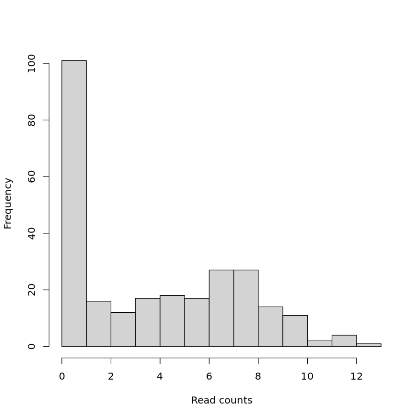
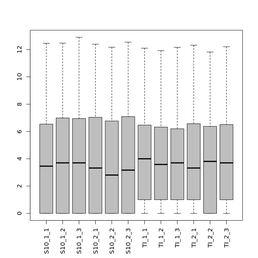
First, we will calculate the “pseudoCounts” as log2 of the reads per gene counts.
This is not part of the actual differential gene expression analysis but is helpful for data exploration and quality assessment. We will look at a histogram of one of the samples and a boxplot representation of the log2 counts for all the 12 samples.
Note that there are many genes with a low number of mapped reads and that there are differences between the average read counts for each library.
pseudoCounts <- log2(DGEList$counts + 1)
head(pseudoCounts)
hist(pseudoCounts[ ,"S10_1_1"], main = "", xlab = "Read counts")
boxplot(pseudoCounts, col = "gray", las = 3, cex.names = 1)| S10_1_1 | S10_1_2 | S10_1_3 | S10_2_1 | S10_2_2 | S10_2_3 | TI_1_1 | TI_1_2 | TI_1_3 | TI_2_1 | TI_2_2 | TI_2_3 | |
|---|---|---|---|---|---|---|---|---|---|---|---|---|
| g175 | 7.169925 | 7.826548 | 7.832890 | 7.768184 | 7.693487 | 7.599913 | 7.876517 | 7.686501 | 7.636625 | 7.794416 | 7.693487 | 7.375039 |
| g176 | 4.169925 | 3.700440 | 4.000000 | 3.169925 | 3.906891 | 4.247928 | 4.906891 | 4.321928 | 4.954196 | 2.807355 | 3.584963 | 4.584963 |
| g178 | 0.000000 | 0.000000 | 0.000000 | 0.000000 | 0.000000 | 0.000000 | 0.000000 | 0.000000 | 1.584963 | 1.584963 | 1.000000 | 1.584963 |
| g180 | 11.437752 | 12.350939 | 12.087131 | 12.015415 | 11.648358 | 12.181463 | 9.988685 | 10.359750 | 9.797662 | 11.385862 | 10.000000 | 11.325305 |
| g181 | 8.888743 | 9.409391 | 9.189825 | 8.774787 | 8.611025 | 8.816984 | 9.328675 | 9.453271 | 9.447083 | 9.346514 | 8.845490 | 8.682995 |
| g182 | 4.321928 | 4.000000 | 4.392317 | 3.321928 | 3.169925 | 2.321928 | 3.807355 | 3.000000 | 3.169925 | 2.807355 | 2.584963 | 2.321928 |
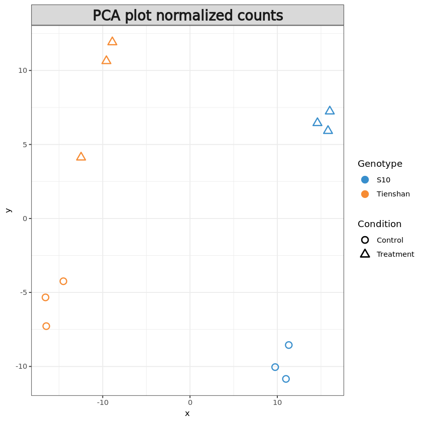
We can also create a PCA plot of the samples in order to assess the differences between the Genotypes and Conditions, but also between the replicates. In this plot the samples that are similar cluster together, while samples that are different are further apart.
In this type of plot, we would expect samples from the same group (the three replicates for each sample) to exhibit a similar gene expression profile thus clustering together while being separated from the other samples.
resPCA <- pca(t(pseudoCounts), ncomp = 6)
plotIndiv(resPCA, group = metadata$Genotype, pch=metadata$Condition,
                  legend = T, legend.title = 'Genotype', legend.title.pch = 'Condition',
                  title = 'PCA plot raw counts', style = 'ggplot2', size.xlabel = 10, size.ylabel = 10)
Warning message in shape.input.plotIndiv(object = object, n = n, blocks = blocks, :
“'ind.names' is set to FALSE as 'pch' overrides it”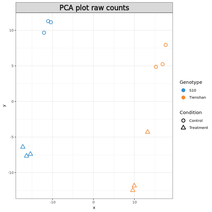
Filtering the lowly expressed genes
As seen previously, many genes have a low number of read counts in our samples. The genes with very low counts across all libraries provide little evidence for differential expression, thus we should eliminate these genes before the analysis.
One of the filtering methods we can use is the “filterByExpr” function provided by the edgeR package. By default, this function keeps only the genes that have at least 10 reads per group, but other cutoffs can also be applied.
keep <- filterByExpr(DGEList, group=metadata$Group) #create the filter
DGEList <- DGEList[keep, , keep.lib.sizes=FALSE] #apply the filter to on the DGEList object
table(keep) #Check the number of genes that passed the filterkeep
FALSE TRUE
104 163 Normalization
As we are working with multiple samples we need to normalize the read counts per gene in order to account for compositional and technical differences between the 12 RNA-seq libraries. For this, we will calculate normalization factors using the trimmed mean of M-values (TMM) method. You can read more about different normalization methods in the user manual.
Note that running “calcNormFactors” does not change the actual reads per gene counts, it just fills the “norm.factors” column in DGEList$samples.
These factors will be used to scale the read counts for each library. From the user guide: “A normalization factor below one indicates that a small number of high count genes are monopolizing the sequencing, causing the counts for other genes to be lower than would be usual given the library size.”
DGEList <- calcNormFactors(DGEList, method="RLE")
DGEList$samples| group | lib.size | norm.factors | Condition | Genotype | |
|---|---|---|---|---|---|
| <fct> | <dbl> | <dbl> | <fct> | <fct> | |
| S10_1_1 | S10_Control | 43506 | 1.0897129 | Control | S10 |
| S10_1_2 | S10_Control | 58660 | 1.0385093 | Control | S10 |
| S10_1_3 | S10_Control | 62512 | 1.0362962 | Control | S10 |
| S10_2_1 | S10_Treatment | 59741 | 0.9802860 | Treatment | S10 |
| S10_2_2 | S10_Treatment | 56653 | 0.8418644 | Treatment | S10 |
| S10_2_3 | S10_Treatment | 63008 | 0.8949144 | Treatment | S10 |
| TI_1_1 | Tienshan_Control | 43174 | 1.0618440 | Control | Tienshan |
| TI_1_2 | Tienshan_Control | 38203 | 1.0431678 | Control | Tienshan |
| TI_1_3 | Tienshan_Control | 40178 | 1.0676351 | Control | Tienshan |
| TI_2_1 | Tienshan_Treatment | 55391 | 0.9048196 | Treatment | Tienshan |
| TI_2_2 | Tienshan_Treatment | 39810 | 1.1235077 | Treatment | Tienshan |
| TI_2_3 | Tienshan_Treatment | 44910 | 0.9603761 | Treatment | Tienshan |
Normalized counts - Exploratory Data analysis
For data analysis purposes normalized log2 counts can be extracted from the DGEList object using the function CPM (counts per million).
We will generate the same plots as for the raw counts in order to compare the data before and after normalization.
Do the plots for normalized counts look different compared with the plots computed before data filtering and normalization?
pseudoNormCounts <- cpm(DGEList, log = TRUE, prior.count = 1)
head(pseudoNormCounts)
hist(pseudoNormCounts[ ,"S10_1_1"], main = "", xlab = "counts")
boxplot(pseudoNormCounts, col = "gray", las = 3, cex.names = 1)
resPCA <- pca(t(pseudoNormCounts), ncomp = 6)
plotIndiv(resPCA, group = metadata$Genotype, pch=metadata$Condition,
legend = T, legend.title = 'Genotype', legend.title.pch = 'Condition',
title = 'PCA plot normalized counts', style = 'ggplot2', size.xlabel = 10, size.ylabel = 10)| S10_1_1 | S10_1_2 | S10_1_3 | S10_2_1 | S10_2_2 | S10_2_3 | TI_1_1 | TI_1_2 | TI_1_3 | TI_2_1 | TI_2_2 | TI_2_3 | |
|---|---|---|---|---|---|---|---|---|---|---|---|---|
| g175 | 11.568005 | 11.864813 | 11.782957 | 11.863090 | 12.083127 | 11.749272 | 12.323049 | 12.334198 | 12.178544 | 12.112851 | 12.175386 | 11.908906 |
| g176 | 8.564108 | 7.760868 | 7.974199 | 7.290213 | 8.292080 | 8.405708 | 9.349782 | 8.956131 | 9.490388 | 7.125494 | 8.054467 | 9.111569 |
| g180 | 15.836359 | 16.387906 | 16.035457 | 16.109276 | 16.038322 | 16.329943 | 14.435626 | 15.008665 | 14.340400 | 15.704307 | 14.482504 | 15.860317 |
| g181 | 13.287211 | 13.446752 | 13.138771 | 12.869139 | 13.000828 | 12.965820 | 13.775545 | 14.101988 | 13.989757 | 13.664955 | 13.327806 | 13.217591 |
| g182 | 8.716557 | 8.056048 | 8.360376 | 7.439590 | 7.551908 | 6.505541 | 8.245462 | 7.611500 | 7.689402 | 7.125494 | 7.041192 | 6.815835 |
| g184 | 9.350249 | 8.573811 | 9.628852 | 9.955925 | 11.089735 | 10.542877 | 9.653135 | 9.546090 | 8.779819 | 11.073313 | 10.609695 | 11.024686 |
Warning message in shape.input.plotIndiv(object = object, n = n, blocks = blocks, :
“'ind.names' is set to FALSE as 'pch' overrides it”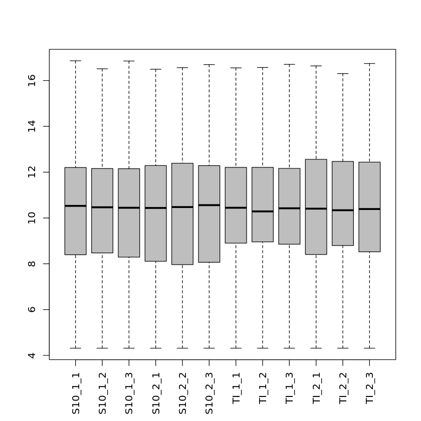
EdgeR - Testing for Differentially expressed genes (DEGs)
We use edgeR for Differential Gene Expression using the GLM method (Generalized linear model) with treatment and genotype effects
After we concluded the exploratory data analysis and the filtering and normalization steps we can now start testing for differentially expressed genes between our samples.
For this, we first need to define a “design matrix” which describes our experimental design. We construct a matrix containing samples as rows and our previously defined groups (S10_Control, S10_Treatment, Tienshan_Control, Tienshan_Treatment) as columns. The samples belonging to each group are assigned a “1” in this matrix.
In few words, the design matrix identifies the various groups between which you can do the differential gene expression test.
design.matrix <- model.matrix(~0+Group)
rownames(design.matrix) <- colnames(DGEList)
colnames(design.matrix) <- levels(metadata$Group)
design.matrix| S10_Control | S10_Treatment | Tienshan_Control | Tienshan_Treatment | |
|---|---|---|---|---|
| S10_1_1 | 1 | 0 | 0 | 0 |
| S10_1_2 | 1 | 0 | 0 | 0 |
| S10_1_3 | 1 | 0 | 0 | 0 |
| S10_2_1 | 0 | 1 | 0 | 0 |
| S10_2_2 | 0 | 1 | 0 | 0 |
| S10_2_3 | 0 | 1 | 0 | 0 |
| TI_1_1 | 0 | 0 | 1 | 0 |
| TI_1_2 | 0 | 0 | 1 | 0 |
| TI_1_3 | 0 | 0 | 1 | 0 |
| TI_2_1 | 0 | 0 | 0 | 1 |
| TI_2_2 | 0 | 0 | 0 | 1 |
| TI_2_3 | 0 | 0 | 0 | 1 |
For easier pairwise comparisons between the groups we can create some “contrasts” using the “makeContrasts” function. This will tell the program which samples we will like to consider as our “Control” and which as our “Treatment” groups. The Control groups will be assigned a “-1” and the Treatment groups a “1”. When using multiple Control and Treatment samples in the same contrast we need to devide by the number of samples used as for example in the contrast S10_Tienshan, where we use both S10 and Ti samples.
For example, the contrast S10 = S10_Treatment - S10_Control will test for differentially expressed genes between the S10 treatment samples vs the S10 Control samples.
contrasts <- makeContrasts(
                S10 = S10_Treatment-S10_Control,
                Tienshan = Tienshan_Treatment-Tienshan_Control,
                S10_Tienshan= (S10_Treatment+Tienshan_Treatment)/2 - (S10_Control+Tienshan_Control)/2,
                levels=design.matrix)
contrasts| S10 | Tienshan | S10_Tienshan | |
|---|---|---|---|
| S10_Control | -1 | 0 | -0.5 |
| S10_Treatment | 1 | 0 | 0.5 |
| Tienshan_Control | 0 | -1 | -0.5 |
| Tienshan_Treatment | 0 | 1 | 0.5 |
- Any ideas for other contrasts that migth be interesting to explore?
The following cell will run two mandatory steps in order to fit a model in edgeR. First, the dispersion needs to be estimated, this is a measure of the degree of inter-library variation for each gene. Afterwards, a QL ( quasi-likelihood) model representing the sample design is fitted using the “glmQLFit” function. You can read more about these steps in the edgeR user guide.
DGEList <- estimateDisp(DGEList, design.matrix)
fit <- glmQLFit(DGEList, design.matrix)
DEGs for White clover S10 plants Treatment vs Control
Find DEGs for White clover S10 plants in Treatment condition compared with the Control condition We will test for differentially expressed genes using the quasi-likelihood F-tests method. This is easily done just by running the “glmQFTest” function on the fit model and selecting one of the contrasts we created above (in this case the “S10” contrast).
Next, we will use the topTags function to extract the information about all the genes.
glmqlf_S10 <- glmQLFTest(fit, contrast=contrasts[,"S10"])
DEG_S10 <- topTags(glmqlf_S10, n = nrow(DGEList$counts))
DEG_S10- $table
-
A data.frame: 163 × 5 logFC logCPM F PValue FDR <dbl> <dbl> <dbl> <dbl> <dbl> g39 3.5861702 14.124630 336.66158 5.227331e-10 8.520550e-08 g232 4.0494125 11.950441 157.50997 3.685988e-08 2.591779e-06 g6 2.3225347 12.999541 150.27854 4.770146e-08 2.591779e-06 g350 2.0530029 13.324566 97.56453 4.890245e-07 1.992775e-05 g99 -1.5387874 11.681004 85.17478 9.976659e-07 3.195090e-05 g142 -1.4235276 13.830692 82.52308 1.176107e-06 3.195090e-05 g240 1.3603712 14.708794 79.98114 1.383201e-06 3.220882e-05 g269 -1.4191681 11.834217 75.66563 1.841279e-06 3.751606e-05 g26 2.1254241 11.366827 68.55898 3.047273e-06 5.518949e-05 g129 -5.3324794 8.679594 60.45459 5.738115e-06 9.353127e-05 g272 3.1405978 13.860652 59.08187 6.432977e-06 9.532503e-05 g157 5.3813801 10.414972 57.03712 7.659515e-06 1.040417e-04 g42 -1.9856547 9.962762 53.97164 1.005146e-05 1.260298e-04 g165 2.2666761 13.690016 51.66777 1.243606e-05 1.447913e-04 g101 3.1488142 13.181625 48.21727 1.736838e-05 1.887363e-04 g15 2.7410696 10.684840 47.29143 1.906062e-05 1.941800e-04 g210 -2.2430064 9.993002 46.52627 2.060621e-05 1.975772e-04 g299 -2.3509276 10.984491 45.75893 2.230566e-05 2.019901e-04 g103 2.6810410 10.579777 44.26963 2.609599e-05 2.238762e-04 g144 -0.7963477 16.186987 43.17707 2.936057e-05 2.392886e-04 g77 1.0984806 14.118231 41.46740 3.548119e-05 2.754016e-04 g125 -1.3099534 10.195970 39.85537 4.266319e-05 3.160955e-04 g298 -2.0471647 9.837072 33.49832 9.395967e-05 6.658881e-04 g104 2.4081173 9.219160 38.54240 1.121281e-04 7.615370e-04 g122 -0.6485441 12.457152 30.90261 1.341148e-04 8.744287e-04 g164 1.4415064 11.156457 30.50383 1.419308e-04 8.897970e-04 g146 1.3983889 12.824184 29.92911 1.541544e-04 9.306356e-04 g313 2.2492040 13.614815 28.41728 1.926822e-04 1.121686e-03 g150 1.9650641 13.229706 27.90020 2.083770e-04 1.171222e-03 g13 -0.6522187 13.101579 26.45593 2.608176e-04 1.417109e-03 ⋮ ⋮ ⋮ ⋮ ⋮ ⋮ g96 -1.873792302 8.939397 0.4844512655 0.4999546 0.6041584 g10 0.233134670 14.382992 0.4834790913 0.5003766 0.6041584 g253 0.052426914 13.741219 0.3075042687 0.5896191 0.7066759 g289 -0.212573283 9.390864 0.2887857862 0.6010328 0.7150974 g312 0.093543041 10.849110 0.2666731965 0.6151559 0.7265972 g301 -0.102000599 10.135184 0.2572520652 0.6214023 0.7274503 g221 -0.277095720 8.469909 0.2522121463 0.6248039 0.7274503 g162 -0.145155616 8.517263 0.2278112475 0.6463283 0.7413085 g50 -0.170907352 8.749274 0.2158314533 0.6507284 0.7413085 g203 0.062836598 14.227601 0.2124612164 0.6532634 0.7413085 g88 0.045949497 14.235850 0.2103049178 0.6548983 0.7413085 g355 -0.287897714 8.890754 0.1803234432 0.6787703 0.7630314 g204 -0.055975779 11.947887 0.1408988543 0.7140799 0.7972262 g306 0.054269738 11.294732 0.0923937800 0.7664733 0.8498990 g193 0.049946343 11.682386 0.0642557849 0.8042743 0.8857886 g205 0.037877227 10.986961 0.0473457745 0.8314821 0.9029713 g194 -0.142990391 9.403497 0.0447552162 0.8360811 0.9029713 g362 0.025629967 11.336529 0.0415198735 0.8420254 0.9029713 g315 0.027958374 11.878331 0.0409766489 0.8430470 0.9029713 g180 0.059680256 15.711409 0.0386140448 0.8475743 0.9029713 g282 -0.026492114 11.756078 0.0247991469 0.8775434 0.9288284 g176 -0.061055115 8.587203 0.0144510429 0.9063467 0.9531258 g126 0.061707217 8.311212 0.0024786868 0.9648334 1.0000000 g128 0.063825269 7.671043 0.0019414812 0.9655950 1.0000000 g227 -0.025740630 7.939955 0.0011908008 0.9730516 1.0000000 g121 0.002660852 12.896620 0.0005233398 0.9821327 1.0000000 g284 0.000000000 8.538720 0.0000000000 1.0000000 1.0000000 g116 0.000000000 7.180297 0.0000000000 1.0000000 1.0000000 g117 0.000000000 7.033307 0.0000000000 1.0000000 1.0000000 g118 0.000000000 7.515646 0.0000000000 1.0000000 1.0000000 - $adjust.method
- 'BH'
- $comparison
- '-1*S10_Control 1*S10_Treatment'
- $test
- 'glm'
We have now created a table with certain parameters calculated for each of the genes analysed.
logFC represents the base 2 logarithm of the fold change and it shows us how much the expression of the gene has changed between the two conditions. A logFC of 1 means a doubling in the read per gene count between the control and treatment samples. The genes with a logFC higher than 0 are upregulated while the genes with a logFC lower than 0 are downregulated between the control and treatment samples.
logCPM represents the average log2-counts-per-million, the abundance of the gene.
F - F-statistic.
PValue is the raw p-value.
FDR (The false discovery rate) represents the adjusted p-value and is calculated using Benjamini and Hochberg’s algorithm. It controls the rate of false positive values under multiple testing. Usually, a threshold of under 5% is set for the FDR.
The important information for us in this table is stored in the “logFC” and the “FDR” columns. The top DE genes have small FDR values and large fold changes
Many of the genes in the samples are uninteresting for us, as they have a high FDR and/or low logFC values so we cannot consider them as differentially expressed.
We will apply a filtering step in order to keep only the statistically significant genes. We will filter out the genes with an FDR higher than 0.05 and an absolute logFC lower than 1.
DEG_S10_filtered <- DEG_S10$table[DEG_S10$table$FDR < 0.05 & abs(DEG_S10$table$logFC) > 1,] #Filtering
DEG_S10_filtered <- rownames_to_column(DEG_S10_filtered) %>% rename(gene_ID = rowname) #Adding the gene_ID column
head(DEG_S10_filtered)
nrow(DEG_S10_filtered) # finding the number of genes that passed the filter | gene_ID | logFC | logCPM | F | PValue | FDR | |
|---|---|---|---|---|---|---|
| <chr> | <dbl> | <dbl> | <dbl> | <dbl> | <dbl> | |
| 1 | g39 | 3.586170 | 14.12463 | 336.66158 | 5.227331e-10 | 8.520550e-08 |
| 2 | g232 | 4.049413 | 11.95044 | 157.50997 | 3.685988e-08 | 2.591779e-06 |
| 3 | g6 | 2.322535 | 12.99954 | 150.27854 | 4.770146e-08 | 2.591779e-06 |
| 4 | g350 | 2.053003 | 13.32457 | 97.56453 | 4.890245e-07 | 1.992775e-05 |
| 5 | g99 | -1.538787 | 11.68100 | 85.17478 | 9.976659e-07 | 3.195090e-05 |
| 6 | g142 | -1.423528 | 13.83069 | 82.52308 | 1.176107e-06 | 3.195090e-05 |
52
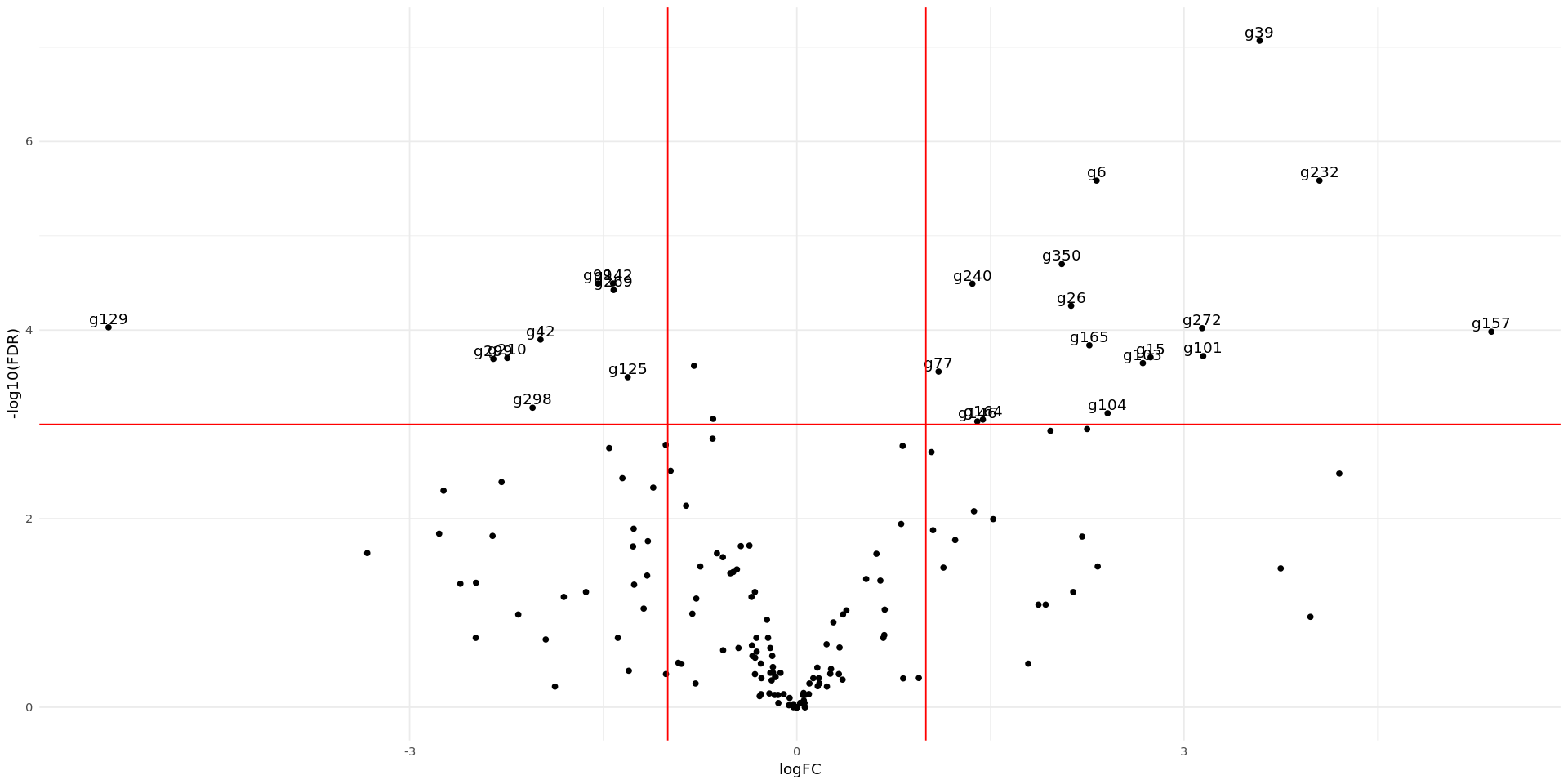
We can also visualize the selected genes by plotting a Volcano plot and a Smear plot. A volcano plot highlits genes that are both significant and have high logFC. In this case, the x-axis is the logFC and the y axis the negative exponent of the p-value. We draw thresholds for -1<logFC<1 and P<0.001. We can see that the majority of the genes analysed are either not statistically significant or have a very small logFC.
We first create a table where we define labels to write on the plot only for genes beyond the defined thresholds.
options(repr.plot.width = 16, repr.plot.height=8)

# adding column for differential expression label
DEG <- DEG_S10$table
DEG <- rownames_to_column(DEG) %>% rename(gene_ID = rowname) #Adding the gene_ID column
DEG$diffexpr <- NA
DEG$diffexpr[(DEG$FDR<0.001)&(abs(DEG$logFC) > 1)] <- DEG$gene_ID[(DEG$FDR<0.001)&(abs(DEG$logFC) > 1)]

ggplot(DEG, aes(x=logFC, y=-log10(FDR), label=diffexpr)) +
  geom_point() +
  theme_minimal() +
  geom_text(aes(label = diffexpr), vjust = -0.3) +
  scale_color_manual(values=c("blue", "black", "red")) +
  geom_vline(xintercept=c(-1, 1), col="red") +
  geom_hline(yintercept=-log10(0.001), col="red")
Warning message: “Removed 138 rows containing missing values or values outside the scale range (`geom_text()`).”
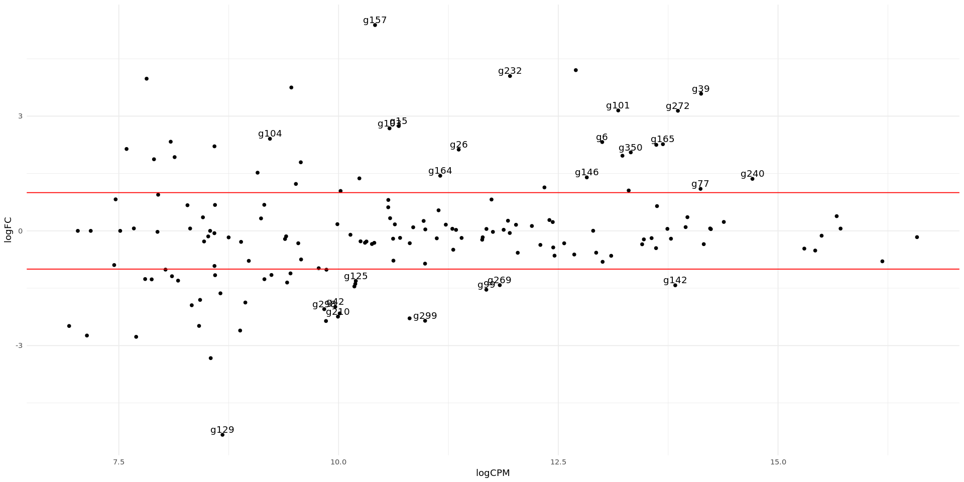
In the smear plot below we have the normalized counts of each gene on the x axis, and the logfold change of each gene on the y axis. Genes which are differentially expressed with many transcripts will show on the right side of the plot and away from the center. The Genes that passed the filter are coloured in red, and the top 10 genes with the lowest FDR value are labelled with their gene ID.
options(repr.plot.width = 16, repr.plot.height=8)

ggplot(DEG, aes(x=logCPM, y=logFC, label=diffexpr)) +
  geom_point() +
  theme_minimal() +
  geom_text(aes(label = diffexpr), vjust = -0.3) +
  scale_color_manual(values=c("blue", "black", "red")) +
  geom_hline(yintercept=c(-1, 1), col="red")
Warning message: “Removed 138 rows containing missing values or values outside the scale range (`geom_text()`).”
We can also create a heatmap with the log2 read counts of the selected differentially expressed genes so that we can visualise the differences in normalized counts between the Control and the Treatment samples.
The genes are ordered by the FDR value.
annot_col <- data.frame(row.names = colnames(pseudoNormCounts)[1:6], Condition = c(rep("Control", 3),rep( "Treatment", 3)))
pheatmap(as.matrix(pseudoNormCounts[DEG_S10_filtered$gene_ID,c(1:6)]), cluster_rows = F, cluster_col = F, annotation_col = annot_col)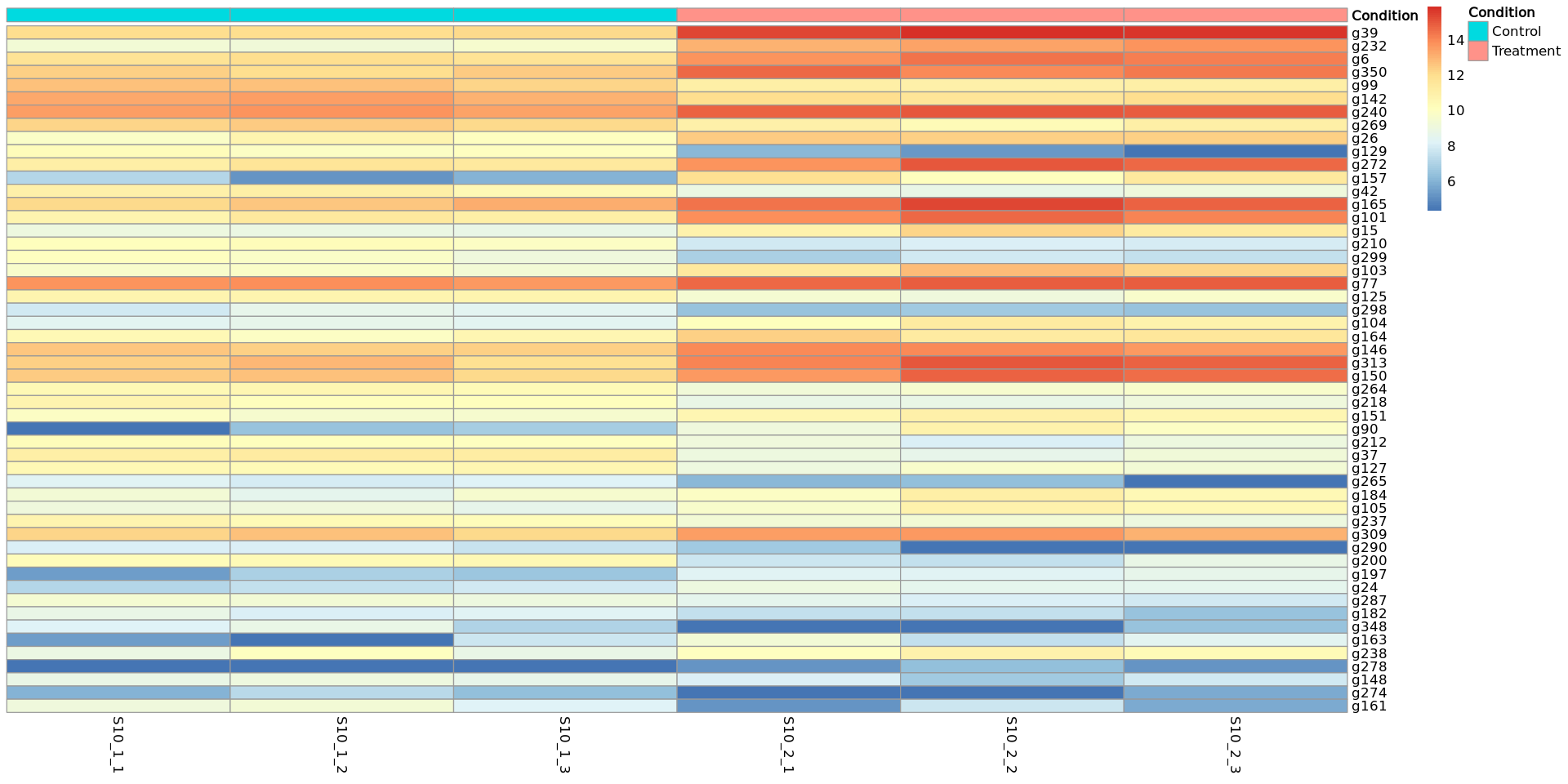
DEGs for White clover Tienshan Treatment vs Control
We can do this using the same functions as above and changing the contrast.
This time we will directly filter the differentially expressed genes using the same parameters as for the S10 samples.
glmqlf_Ti <- glmQLFTest(fit, contrast=contrasts[,"Tienshan"])
DEG_Ti <- topTags(glmqlf_Ti, n = nrow(DGEList$counts))
DEG_Ti_filtered <- DEG_Ti$table[DEG_Ti$table$FDR < 0.05 & abs(DEG_Ti$table$logFC) > 1,]
DEG_Ti_filtered <- rownames_to_column(DEG_Ti_filtered) %>% rename(gene_ID = rowname)
print(head(DEG_Ti_filtered))
print("Nr of differentially expressed genes:")
print(nrow(DEG_Ti_filtered))
gene_ID logFC logCPM F PValue FDR
1 g234 -3.348667 13.00417 278.01679 1.547626e-09 2.522630e-07
2 g269 -1.885843 11.83422 127.39949 1.172628e-07 9.556922e-06
3 g26 2.423725 11.36683 74.33983 2.016212e-06 8.910761e-05
4 g101 4.303290 13.18162 73.17140 2.186690e-06 8.910761e-05
5 g272 3.391225 13.86065 66.80131 3.475790e-06 9.840357e-05
6 g99 -1.430395 11.68100 66.25814 3.622217e-06 9.840357e-05
[1] "Nr of differentially expressed genes:"
[1] 42We can now plot a Venn diagram with the DEGs for the two genotypes in order to observe the number of common and specific differentially expressed genes between the two genotypes as response to the cold exposure. You can see that a high percentage of the identified genes are common for the two genotypes, while each genotype has also specific genes.
vd <- venn.diagram(
  x = list(DEG_S10_filtered$gene_ID, DEG_Ti_filtered$gene_ID),
  category.names = c("S10" , "Tienshan"),
  lwd = 4,
  fill = c("cornflowerblue", "yellowgreen"),
  filename = NULL,
  cat.cex = 1,
  cat.fontface = "bold",
  output=TRUE
)
grid.draw(vd)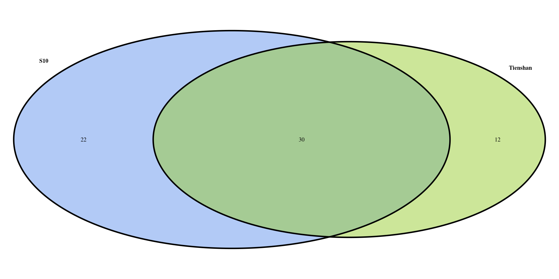
DEGs for S10+Tienshan Treatment vs Control w/o genotype effects
Until now we tested for DEGs specific for each of the two genotypes under cold treatment. We can also run a test where we ignore the genotype and just test for the differences in the cold response.
Consider the counts for both genotypes as a single dataset using the previously created contrast “S10_Tienshan”.
* Do the results look different compared with the previous tests?
glmqlf_S10_Ti <- glmQLFTest(fit, contrast=contrasts[,"S10_Tienshan"])
DEG_S10_Ti <- topTags(glmqlf_S10_Ti, n = nrow(DGEList$counts))
DEG_S10_Ti_filtered <- DEG_S10_Ti$table[DEG_S10_Ti$table$FDR < 0.05 & abs(DEG_S10_Ti$table$logFC) > 1,]
DEG_S10_Ti_filtered <- rownames_to_column(DEG_S10_Ti_filtered)  %>% rename(gene_ID = rowname)
print(head(DEG_S10_Ti_filtered))
print("Nr of differentially expressed genes:")
print(nrow(DEG_S10_Ti_filtered))
gene_ID logFC logCPM F PValue FDR
1 g39 2.057128 14.12463 246.6519 3.039491e-09 4.954370e-07
2 g232 3.261008 11.95044 203.4580 8.934889e-09 5.288546e-07
3 g269 -1.652505 11.83422 200.3564 9.733520e-09 5.288546e-07
4 g6 1.714849 12.99954 166.2297 2.740066e-08 1.116577e-06
5 g99 -1.484591 11.68100 150.3246 4.762148e-08 1.552460e-06
6 g26 2.274575 11.36683 142.8625 6.290957e-08 1.623160e-06
[1] "Nr of differentially expressed genes:"
[1] 52Plot the results from the 3 tests in a Venn diagram to visualize the number of common and unique genes
vd <- venn.diagram(
  x = list(DEG_S10_filtered$gene_ID, DEG_Ti_filtered$gene_ID,
           DEG_S10_Ti_filtered$gene_ID),
  category.names = c("S10" , "Tienshan", "S10_Tienshan"),
  lwd = 3,
  fill = c("cornflowerblue", "yellowgreen", "thistle3"),
  filename = NULL,
  cat.cex = 1,
  cat.fontface = "bold",
  output=TRUE
)
grid.draw(vd)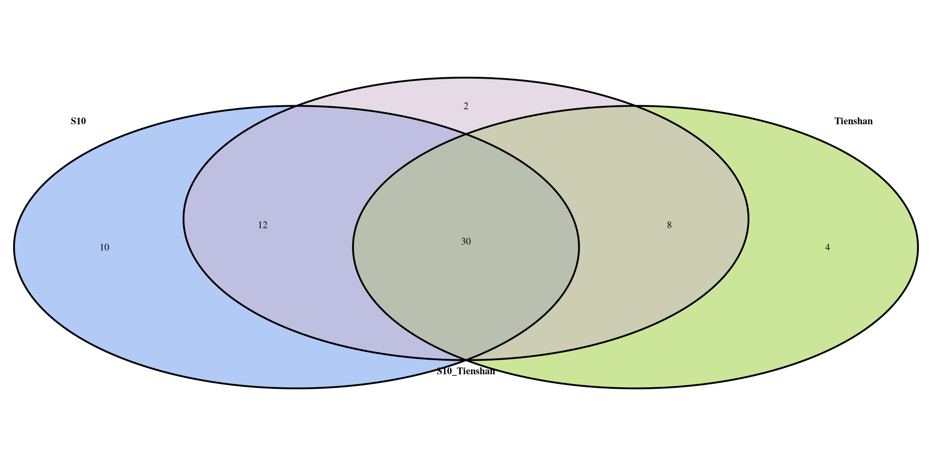
Explore DGE results
Select the genes which appear only in the analysis using both genotypes for further examination.
We can use the “anti_join” function from the dplyr package to keep only the unique genes that appear only when using both genotypes.
S10_Ti_unique <- anti_join(DEG_S10_Ti_filtered, DEG_S10_filtered, by="gene_ID") %>%
                       anti_join(DEG_Ti_filtered, by="gene_ID")
S10_Ti_unique| gene_ID | logFC | logCPM | F | PValue | FDR |
|---|---|---|---|---|---|
| <chr> | <dbl> | <dbl> | <dbl> | <dbl> | <dbl> |
| g247 | -1.412652 | 8.424523 | 10.877350 | 0.006535994 | 0.01500517 |
| g360 | 1.180849 | 7.900076 | 9.804067 | 0.013809376 | 0.02813660 |
Linking the genes selected as differentially expressed back to the raw read counts
How do the counts look for these genes, does it make sense that they are differentially expressed only when using the two genotypes?
Read_counts <- rownames_to_column(Read_counts) %>% rename(gene_ID = rowname)
S10_Ti_unique_counts <- inner_join(S10_Ti_unique[,c(1,2,6)], Read_counts, by="gene_ID")
S10_Ti_unique_counts| gene_ID | logFC | FDR | S10_1_1 | S10_1_2 | S10_1_3 | S10_2_1 | S10_2_2 | S10_2_3 | TI_1_1 | TI_1_2 | TI_1_3 | TI_2_1 | TI_2_2 | TI_2_3 |
|---|---|---|---|---|---|---|---|---|---|---|---|---|---|---|
| <chr> | <dbl> | <dbl> | <int> | <int> | <int> | <int> | <int> | <int> | <int> | <int> | <int> | <int> | <int> | <int> |
| g247 | -1.412652 | 0.01500517 | 4 | 9 | 3 | 1 | 2 | 1 | 42 | 27 | 32 | 8 | 22 | 22 |
| g360 | 1.180849 | 0.02813660 | 1 | 0 | 1 | 3 | 2 | 3 | 16 | 10 | 16 | 22 | 19 | 22 |
Adding functional annotation to DEGs
Until now we looked only at gene IDs, but we can also add functional annotations to the DEGs. The functional annotations were generated using protein sequences and the EggNOG software.
Identifying the molecular function of the differentially expressed genes can help us do a literature survey in order to check if any of the genes discovered have been previously identified as being involved in the cold response.
Functional_annotations <- read.delim("../Data/Clover_Data/Functional_Annotations.txt")
S10_Ti_unique_FA <- inner_join(S10_Ti_unique[,c(1,2,6)], Functional_annotations, by="gene_ID")
S10_Ti_unique_FA| gene_ID | logFC | FDR | Human.Readable.Description |
|---|---|---|---|
| <chr> | <dbl> | <dbl> | <chr> |
| g247 | -1.412652 | 0.01500517 | Nitrogen regulatory protein P-II homolog |
| g360 | 1.180849 | 0.02813660 | Unknown protein |
Task:
- Based on the results obtained in the analysis so far, would you change the cut-off for the FDR and logFC to be more strict or more permissive? Look back at the raw counts for different FDR and logFC values and set the thresholds as you find appropriate.
You can also plot histograms with the FDR and logFC values.
hist(DEG_S10$table$FDR , main = "", xlab = "FDR", breaks= 200, xlim = range(c(0, 0.1)))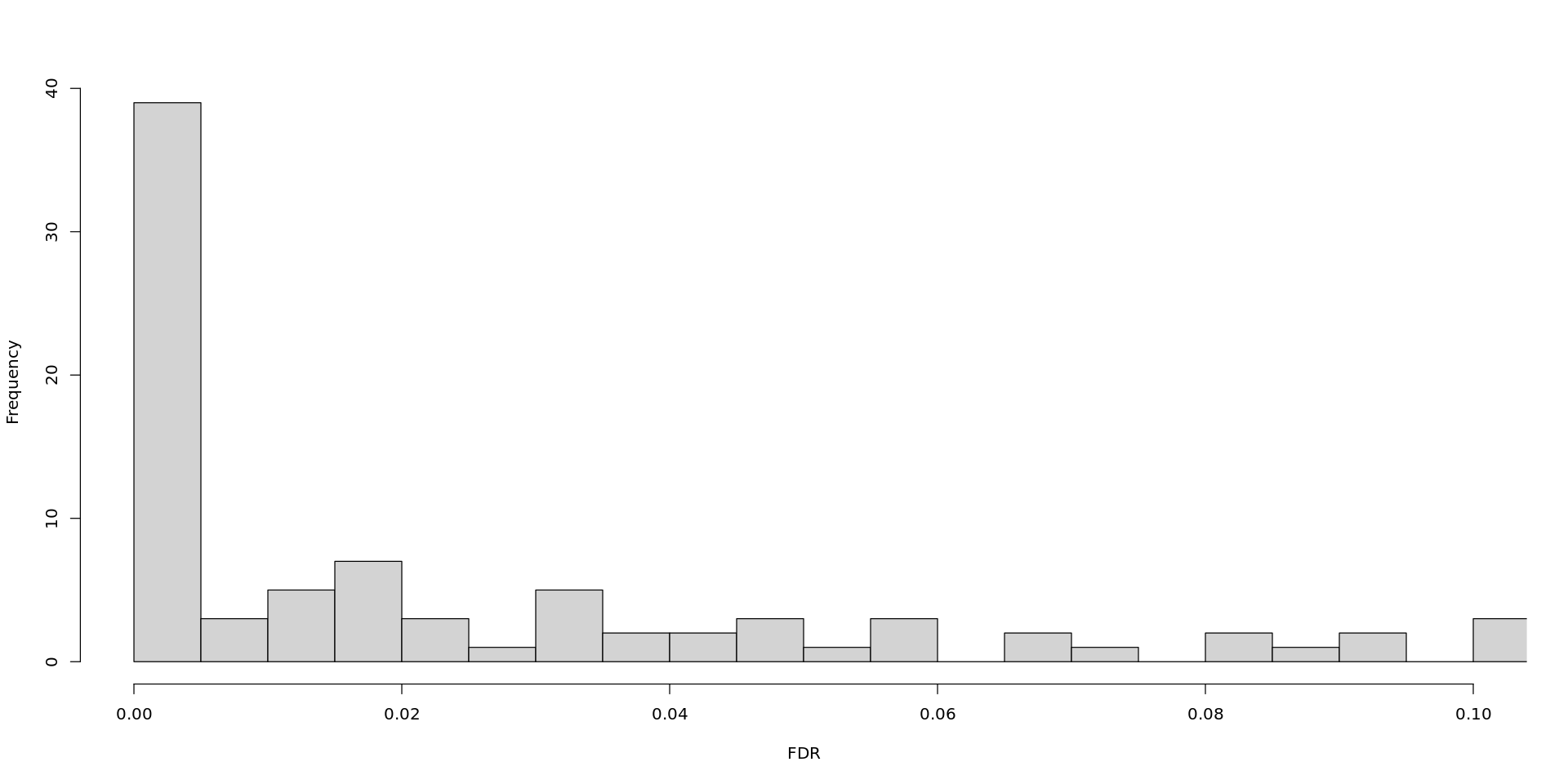
hist(DEG_S10$table$logFC , main = "", xlab = "logFC", breaks= 50, xlim = range(c(-6, 6)))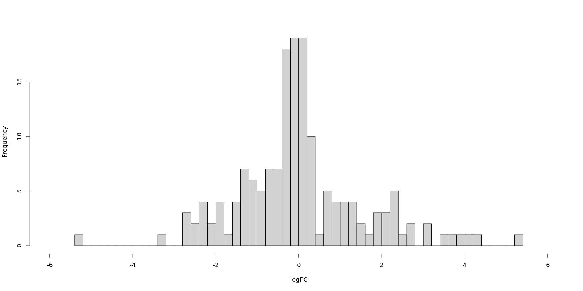
- Separate the upregulated and downregulated genes for each genotype and append functional annotations to them.
- Identify the genes that are commonly upregulated in S10 and Tienshan samples and the uniquely upregulated genes for each genotype.
- Why do you think some of the proteins appear in duplicates?
To answer these questions, it may be convenient to save summary tables from R and open them in excel. See the code below for examples of how to do this. Files can be downloaded by right-clicking on the file name.
If you are familiar with R functions, you are welcome to use those for counting.
dir.create("DEG_Output_tables", showWarnings = FALSE)#Create the table with the DEGs, Raw counts(just for the Ti samples in this case, change to columns (2:7) for the S10 samples) and Functional annotations
DEG_Ti_counts_FA <- inner_join(DEG_Ti_filtered[,c(1, 2, 6)], Read_counts[, c(1, 8:13)], by="gene_ID") %>%
inner_join(Functional_annotations, by="gene_ID")
#Write the table to file
write.table(DEG_Ti_counts_FA, file = "DEG_Output_tables/Ti_Treatment_Control_DGE.txt", quote = FALSE, row.names = FALSE, sep = "\t")
#Display the first 10 rows of the table
head(DEG_Ti_counts_FA, n=10)| gene_ID | logFC | FDR | TI_1_1 | TI_1_2 | TI_1_3 | TI_2_1 | TI_2_2 | TI_2_3 | Human.Readable.Description | |
|---|---|---|---|---|---|---|---|---|---|---|
| <chr> | <dbl> | <dbl> | <int> | <int> | <int> | <int> | <int> | <int> | <chr> | |
| 1 | g234 | -3.348667 | 2.522630e-07 | 1189 | 1515 | 1080 | 131 | 123 | 146 | Polysaccharide lyase family 4, domain III |
| 2 | g269 | -1.885843 | 9.556922e-06 | 289 | 237 | 259 | 79 | 74 | 74 | zinc finger |
| 3 | g26 | 2.423725 | 8.910761e-05 | 22 | 23 | 34 | 202 | 160 | 100 | Transcription factor PIF3 |
| 4 | g101 | 4.303290 | 8.910761e-05 | 17 | 39 | 39 | 1138 | 279 | 664 | WRKY transcription factor 23 |
| 5 | g272 | 3.391225 | 9.840357e-05 | 87 | 133 | 145 | 2121 | 702 | 1391 | WRKY transcription factor 23 |
| 6 | g99 | -1.430395 | 9.840357e-05 | 160 | 136 | 146 | 77 | 57 | 43 | zinc finger |
| 7 | g232 | 2.472603 | 1.660786e-04 | 26 | 40 | 13 | 164 | 189 | 123 | Retrovirus-related Pol polyprotein from transposon TNT 1-94 |
| 8 | g240 | 1.107904 | 1.829713e-04 | 781 | 884 | 964 | 2546 | 1740 | 1865 | Shaggy-related protein kinase alpha |
| 9 | g90 | 4.610490 | 2.085299e-04 | 22 | 39 | 66 | 1833 | 361 | 1226 | Galactinol synthase 1 |
| 10 | g92 | -1.331468 | 2.394810e-04 | 216 | 183 | 191 | 89 | 83 | 79 | F-box/LRR-repeat protein At3g26922 |
Example for filtering and counting the Up/Down genes. You can easily filter using the “filter()” function just by specifying the dataframe and a logical argument.
DEG_Ti_up <- filter(DEG_Ti_counts_FA, logFC > 0)
print("Nr of upregulated genes:")
print(nrow(DEG_Ti_up))
DEG_Ti_down <- filter(DEG_Ti_counts_FA, logFC < 0)
print("Nr of downregulated genes:")
print(nrow(DEG_Ti_down))
[1] "Nr of upregulated genes:"
[1] 22
[1] "Nr of downregulated genes:"
[1] 20You can use the “inner_join” and the “anti_join” functions from the dplyr package to select the common and unique genes for each genotype:
example_file_joined <- inner_join(file1, file2, by="gene_ID")
End of the task
Wrapping up
In this notebook, you have worked with RNA-seq results for two white clover genotypes exposed to one night of cold treatment, aiming to identify genes that change their expression in response to the cold treatment. You have learned to perform exploratory data analysis of raw and normalized RNA-seq read counts. You have also performed differential gene expression using edgeR.
Do you want to look for more analysis? We have an introductory course on bulkRNA analysis at the Danish Health Data Science Sandbox (held periodically in Copenhagen, keep an eye on the webpage where they list courses). You can also find the material on the Transcriptomics Sandbox on uCloud (for danish users of uCloud), otherwise the course is documented in web format at the respective webpage.