Quality Control and Alignment of raw reads
This first exercise will be executed on Galaxy, an interactive platform to run bioinformatics workflows. We will replicate this lesson with computer code later in this course. Galaxy has the possibility of working with a free account.
Biological introduction
White clover (Trifolium repens) is an allotetraploid. This means that it contains genomes originating from two different species within the same nucleus. Normally, white clover is an outbreeding species, but a self-compatible line was used for sequencing the white clover genome. This line is designated S10 in your data, indicating that this is the 10th self-fertilized generation. In addition, you have data from a wild clover accession (ecotype) called Tienshan (Ti), which is collected from Chinese mountains and is adapted to alpine conditions.
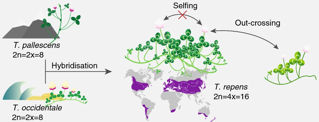 Figure: Characterisation of the white clover population. T.Repens is a hybrid of T.Occidentale and T.Pallescens
Exercise guide
Prepare the tools and data
- Install IGV on your computer from here. This is a genome browser you will use to look at some files.
- Create an account at usegalaxy.org and log into galaxy.
- Find the course data by going to this web address and by clicking on Import this history (top left corner of the page).
If usegalaxy.org has availability problems, you can use the other server https://usegalaxy.eu/ and get the data at this link. You might need to create an account there as well.
Data
You will be working with two types of sequencing data. The first is PacBio Hifi reads, which are long and accurate. You can find them under Hifi_reads_white_clover.fastq. The second type is Illumina RNA-seq reads, which are short and accurate and should be aligned using a spliced aligner, such as STAR.
There are 24 of these files, 12 for each of the two genotypes mentioned before. The files are named [genotype]_[treatment]_[replicate].fastq. Treatment 1 is before and treatment 2 is after exposure to frost, respectively.
In addition to the sequencing data, there are also three reference files: one for homologous contig 1 (referencing T. occidentale-derived subgenome), one for contig 2 (T. pallescens-derived subgenome) and one for both Contigs 1 and 2. The reference files are in fasta format.
The file white_clover_genes.gtf contains the gene annotations for the two contigs.
Workflow illustration
Through Galaxy, we build a workflow applying tools to the data. We will look at the quality of the raw reads for both PacBio HiFi and Illumina RNA-seq reads. Afterwards, we align to references, using two different tools for the two types of data. Finally, we will look at the alignments on a genome browser. We will work then on a computing cluster to analyze the aligned data in some of the upcoming lessons of the course. The computing cluster is necessary because the analysis requires more resources than the ones offered for free by Galaxy.
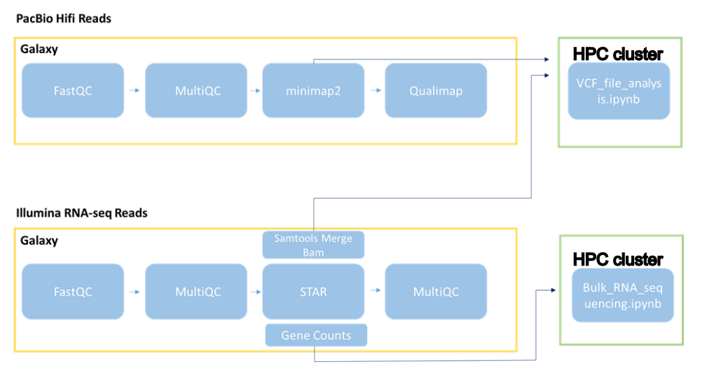
Galaxy Workflow
When you import the files, what you actually import is a History - a sequence of files and softwares applied on the data. You can see the history on the right side of your usegalaxy.org webpage with green panels. Here, we only have the starting data, and you will build the rest of your history through various tools.
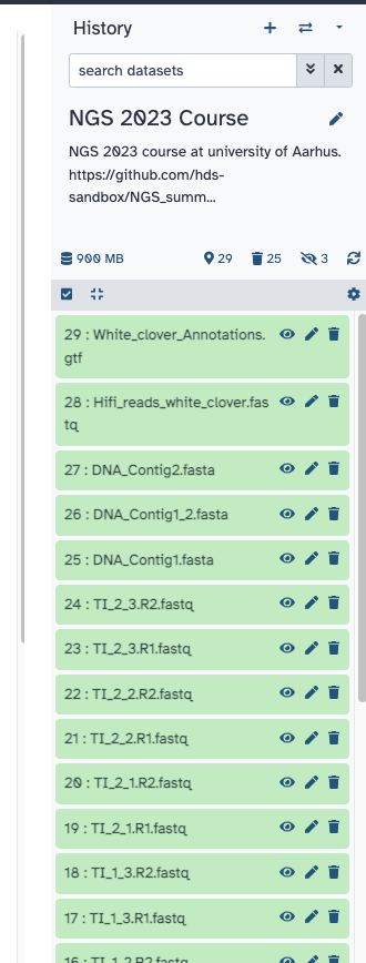
On the left side of the screen, you have a menu with various available tools organized by category. All those softwares are also available on a classical computing command line (we will try those as well).

There are quite many tools in Galaxy. Please use the search bar above the toolbar to find quickly the programs we need.
Quality control
1 Run FastQC on the PacBio Hifi reads and on two of the Illumina RNA-seq libraries. FastQC does quality control of the raw sequence data, providing an overview of the data which can help identify if there are any problems that should be addressed before further analysis.
In the tool searchbar, find FastQC and choose FASTQC read quality reports. You will see a window with tool parameters: for the first option (raw read data from your current history), choose multiple files and select Hifi_reads_white_clover.fastq plus other fastq files you want to see the quality of (example in figure below). Then click on the button Run Tool. 
You will notice that some new elements are added to your history. Part of them are FastQC producing a text file, while others are FastQC producing a webpage report. The reports are ready when coloured in green: click on the eye symbol of a history item to read a report.
2 FastQC provides a report for each sample. To have a better comparison between the Hifi and Illumina data, we would combine the three FastQC reports into one using MultiQC.
Find the tool called MultiQC aggregate results from [...]. In the options, select FastQC as the used tool for the generated logs. Then select the items of FastQC of your history producing RawData (Figure below). In this way, you build a pipeline from the previous reports to the new tool you are using. Now click on Run Tool.
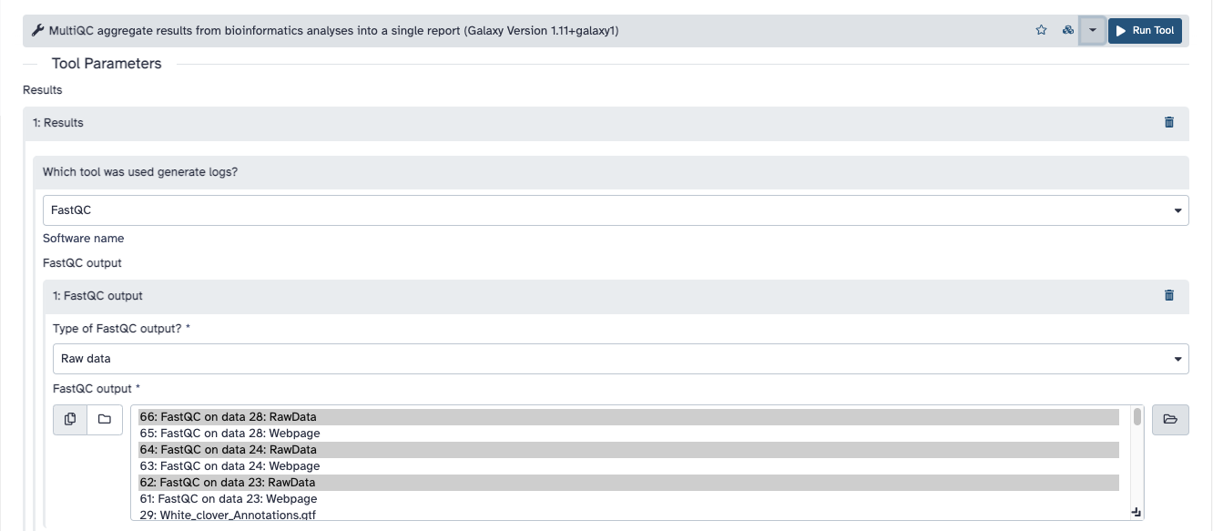
The tool will be now running in your history. When it is done, click on the eye symbol to see the report.
You can find a “Help” button that offers additional information about the plots for each panel.
Focus on the following panels: “Per base sequence quality”, “Per sequence quality scores”…. (“Per base sequence content” always gives a FAIL for RNA-seq data). What do you notice with respect to the sequence quality scores? And are there any other quality issues worth noting?
Hifi Data Alignment
3 Map the PacBio Hifi reads (Hifi_reads_white_clover.fastq) to the white clover reference sequence (Contigs 1 and 2) using minimap2 (Map with minimap2). Find the minimap2 tool. In the options, change Use a built-in genome index into but select the option for having a genome from history and build an index from that. Choose then DNA_Contig1_2.fasta as the reference sequence.
Under the profile with preset options, choose PacBio HiFi reads vs reference mapping (map-hifi). Then click on Run Tool.
4 Run the same alignment, but choose as preset options Long assembly to reference mapping. Up to 20% divergence (asm20).
Rename then the two alignments using the edit function (pen symbol in the history). Use for example names Contig1_2_maphifi and Contig1_2_asm20, to distinguish alignment options and reference genome.
5 The aligned genomes are not sorted by coordinates. Sort the alignments using Samtools sort. In the options, choose the two aligned files with multiple selection. Then click on Run Tool.
6 Download the two alignments to your computer. To do so, click on the disk symbol of each file in your history, and for each download both the Dataset (alignments in bam format) and their index files (in bai format). Download as well the reference genome in fasta format (DNA_Contig1_2.fasta from the history).
7 Open IGV on your computer. Load the reference first: go on Genome --> Load genome from file and select the fasta file you downloaded. Then load the two alignments: go on File --> Load from file and select the bam and bai files you downloaded, together. You can now visualize the alignments by choosing a region of the genome and zooming in.
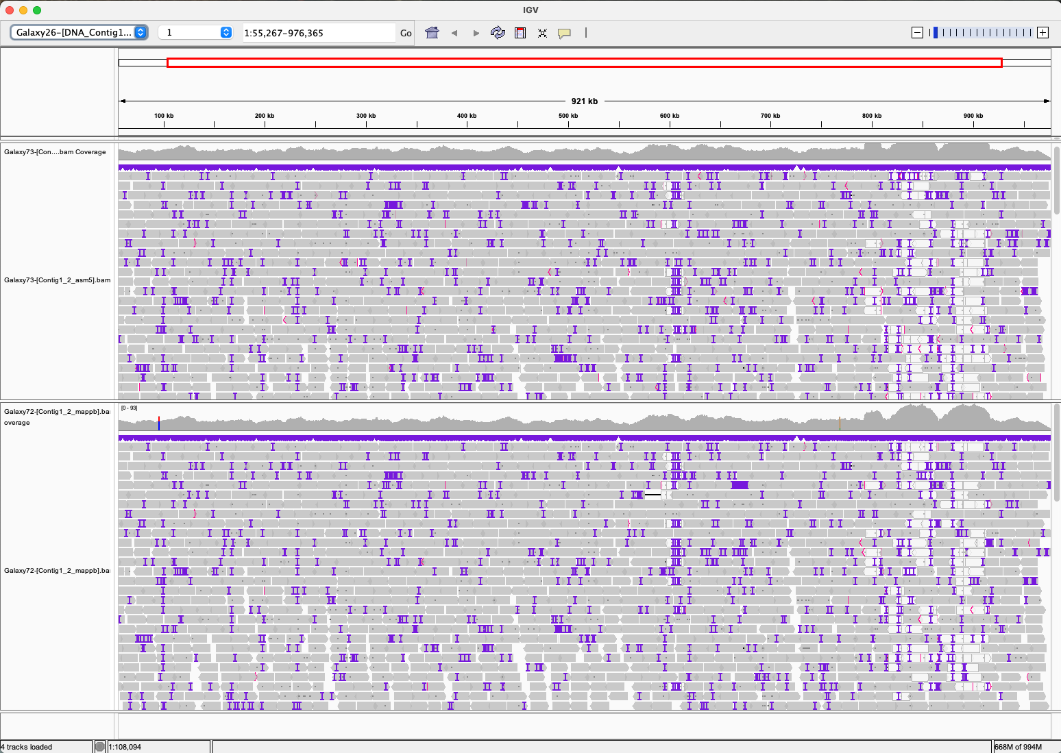
Look at the alignments in IGV. What do you notice about the alignments? What is the difference between the two alignments? Do you think one of them is better than the other? Choose on of the two alignments for the next steps.
8 Repeat the alignment with Minimap2 (using the chosen alignment option from the question above) and the sorting, but using the reference genomes for Contig 1 and for Contig 2 searaately. Note: you can run all at once by choosing multiple reference genomes in the options!
Download the two references for Contig 1 and 2, and the two sorted alignments. Load the references from the menu Genomes in IGV, and then open the two alignments using the menu File in IGV.
Why do you see fluctuations in coverage and large regions without any apparent subgenome SNPs?
What are the major differences between the stats for the reads mapped to Contigs1&2 versus contig1 and contig2? What is your interpretation of the differences?
RNA Data Alignment
9 First, group the 24 RNA-seq libraries into two dataset lists, one list of pairs for S10 libraries and another for Tienshan libraries. so we can work with multiple samples simultaneously. You can do this by selecting the libraries for each genotype and choosing Build Lists of Dataset Pairs.

The grouping suggested by Galaxy is wrong, because the paired reads are paired according to _1 and _2 in their names. Change those two with R1 and R2, click on Unpair all, and then click on the suggested corrected pairs with the buttons Pair these datasets.
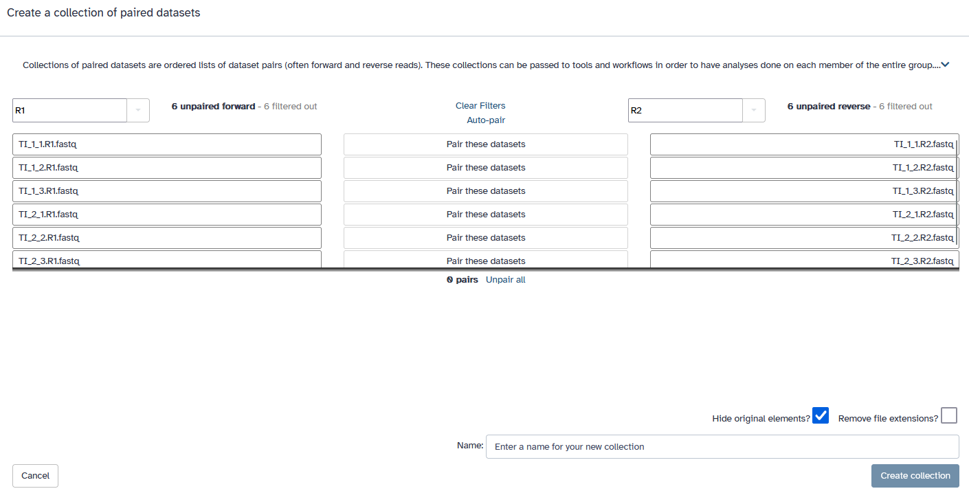
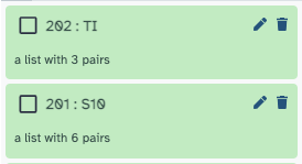
Your sequences will be substituted by two elements in your history. Here we chose for example to name them S10 and TI.
10 Do alignment of the RNA-seq lists of raw files to the reference DNA_Contig1_2.fasta using STAR Gapped-read mapper for RNA-seq data. In the options use:
- as data, the parameter
Paired-end (as collection), and then choose one of the two collections (you cannot run them all at once) - as reference,
DNA_Contig1_2.fasta, with Length of SA pre-indexing string equal to9 - as index with gene-model, use
white_clover_genes.gtf - as output,
Per gene read counts (GeneCounts).
11 Use MultiQC to see the quality of the output. The alignment of STAR produces log files which can be used for quality reports. In the options of MultiQC select the tool STAR. Then Insert STAR output, as type of output the Log, and choose the two logs listing collections of STAR alignments. Then click on Run Tool.

View the report to see the alignment statistics.
Galaxy can also be used to create an automatic workflow that will map the data. This workflow can be useful when running multiple samples. You can generate a workflow from the analysis already completed in a history, by going to Settings → Extract workflow. You can also create a workflow from scratch using the Workflow editor.