mkdir -p Results/GWAS6

# Create two links to data
ln -sf ../DataPolygenic scores I
Important notes for this notebook
Polygenic scores (PRS) estimate an individual’s genetic predisposition to complex traits or diseases by combining information from multiple genetic variants previously identified in the GWAS study. This notebook provides a step-by-step guide to performing a basic PRS analysis using PRSice and explains how to interpret the results.
Learning outcomes
- Discuss and choose the PRS equation
- Discuss PRS scores and biases
How to make this notebook work
- In this notebook, we will only use the
bash command line. Be sure to click on the menuKernel --> Change Kernel --> Bash
 Choose the Bash kernel
While most individual associations found in GWAS studies are of small effect, information about them can be combined across the genome, to create a polygenic score (PGS). These scores can be used to make genome-based predictions about the overall risk of having a particular trait or disease or about the genetic value for continuous traits. If the prediction is on a discrete phenotype such as a disease, these scores are known as polygenic risk scores (PRS).
Polygenic risk prediction analyses
Single-variant association analysis has been the foundation of GWAS. However, detecting more than a handful of significant SNPs for many complex traits requires extremely large sample sizes. In contrast, PGS aggregate genetic risk across multiple variants into a single polygenic score for a given trait.
A PGS is typically calculated by summing the allele frequencies of statistically significant trait-associated variants, weighted by their effect sizes, while ensuring independence among them (e.g., via LD pruning). These effect sizes—betas for continuous traits and log odds ratios for binary traits—are obtained from a discovery GWAS. Large discovery samples (also known as base or training samples) are needed for accurate estimates, but if the target sample shares ancestry, effect sizes from larger studies can be leveraged. A target sample of ~2,000 individuals may be sufficient to detect meaningful genetic contributions to trait variance (Dudbridge 2013). For many complex traits, SNP effect sizes are publicly available (e.g., see https://www.nealelab.is/uk-biobank, https://www.med.unc.edu/pgc/downloads or https://www.ebi.ac.uk/gwas/).
A common practice to calculate PRS involves clumping GWAS results using p-value thresholds (e.g., p < 0.05) to exclude poorly associated SNPs. Usually, multiple PRS analyses will be performed, with varying thresholds for the p-values of the association test.
Once PRS are calculated, they are used in (logistic) regression models to assess the contribution to the trait variance. Prediction accuracy is measured by the increase in \(R^2\), comparing a baseline model with only covariates (e.g., MDS components) to a model that also includes PRS. This increase reflects the proportion of variance explained by genetic risk factors. Accuracy depends on trait heritability, SNP count, and discovery sample size, with a few thousand individuals typically sufficient for reliable estimates.
Polygenic risk score analysis with PRSice-2
PRSice is a widely used tool for polygenic risk score analysis. This tutorial offers a step-by-step guide on its use and result interpretation.
The installed package will include an R script that is straightforward to run. It requires the following information:
--prsice: the binary executable file--base: the.assocfile that contains statistical information--target: the PLINK-formatted dataset
Note
We would apply this method to our HapMap dataset, but PRS analysis typically requires a sample size of around 2,000 to produce meaningful results, while our dataset includes only about 150 individuals. To facilitate learning, we will instead use a toy dataset. In this notebook, we will focus on analyzing a binary trait.
Ideally, the summary statistics should come from the most powerful GWAS available for the phenotype of interest. Commonly, the target dataset is typically generated within your lab or obtained through collaborations.
PRSice analysis for binary traits
![]() Let’s create a folder for the output files. Then, perform the PRS analysis on the toy dataset in the following way:
Let’s create a folder for the output files. Then, perform the PRS analysis on the toy dataset in the following way:
We will run the PRSice.R script using the association test results (TOY_BASE_GWAS.assoc) and specify the column names for SNPs, chromosomes, and other relevant data. This is necessary because different association tools generate varying header formats. Finally, we will specify the location of our data (TOY_TARGET_DATA) and define the phenotype format as binary (0s and 1s).
Warning
If you get an error in the following command, try to restart the kernel in the Kernel menu. Sometimes links to folders are not recognized immediately.
# Recommendation: check the usage instructions and mandatory input files by uncommenting the command below:
#PRSice -h
PRSice --base ./Data/TOY_BASE_GWAS.assoc \
--snp SNP --chr CHR --bp BP --A1 A1 --A2 A2 --stat OR --pvalue P \
--target ./Data/TOY_TARGET_DATA \
--out Results/GWAS6/PRSice \
--binary-target TPRSice 2.3.5 (2021-09-20)
https://github.com/choishingwan/PRSice
(C) 2016-2020 Shing Wan (Sam) Choi and Paul F. O'Reilly
GNU General Public License v3
If you use PRSice in any published work, please cite:
Choi SW, O'Reilly PF.
PRSice-2: Polygenic Risk Score Software for Biobank-Scale Data.
GigaScience 8, no. 7 (July 1, 2019)
2025-03-20 14:03:50
PRSice \
--a1 A1 \
--a2 A2 \
--bar-levels 0.001,0.05,0.1,0.2,0.3,0.4,0.5,1 \
--base ./Data/TOY_BASE_GWAS.assoc \
--binary-target T \
--bp BP \
--chr CHR \
--clump-kb 250kb \
--clump-p 1.000000 \
--clump-r2 0.100000 \
--interval 5e-05 \
--lower 5e-08 \
--num-auto 22 \
--or \
--out Results/GWAS6/PRSice \
--pvalue P \
--seed 2840029482 \
--snp SNP \
--stat OR \
--target ./Data/TOY_TARGET_DATA \
--thread 1 \
--upper 0.5
Initializing Genotype file: ./Data/TOY_TARGET_DATA (bed)
Start processing TOY_BASE_GWAS
==================================================
Base file: ./Data/TOY_BASE_GWAS.assoc
Header of file is:
SNP CHR BP A1 A2 P OR
Reading 32.60%IOPub message rate exceeded.
The Jupyter server will temporarily stop sending output
to the client in order to avoid crashing it.
To change this limit, set the config variable
`--ServerApp.iopub_msg_rate_limit`.
Current values:
ServerApp.iopub_msg_rate_limit=1000.0 (msgs/sec)
ServerApp.rate_limit_window=3.0 (secs)
Reading 74.31%IOPub message rate exceeded.
The Jupyter server will temporarily stop sending output
to the client in order to avoid crashing it.
To change this limit, set the config variable
`--ServerApp.iopub_msg_rate_limit`.
Current values:
ServerApp.iopub_msg_rate_limit=1000.0 (msgs/sec)
ServerApp.rate_limit_window=3.0 (secs)
Reading 100.00%
91062 variant(s) observed in base file, with:
2226 variant(s) located on haploid chromosome
88836 total variant(s) included from base file
Loading Genotype info from target
==================================================
2000 people (1024 male(s), 976 female(s)) observed
2000 founder(s) included
Warning: Currently not support haploid chromosome and sex
chromosomes
88836 variant(s) included
There are a total of 1 phenotype to process
Start performing clumping
Clumping Progress: 100.00%
Number of variant(s) after clumping : 88836
Processing the 1 th phenotype
Phenotype is a binary phenotype
1000 control(s)
1000 case(s)
Start Processing
Processing 40.15%
IOPub message rate exceeded.
The Jupyter server will temporarily stop sending output
to the client in order to avoid crashing it.
To change this limit, set the config variable
`--ServerApp.iopub_msg_rate_limit`.

Current values:
ServerApp.iopub_msg_rate_limit=1000.0 (msgs/sec)
ServerApp.rate_limit_window=3.0 (secs)
Processing 100.00%
There are 1 region(s) with p-value less than 1e-5. Please
note that these results are inflated due to the overfitting
inherent in finding the best-fit PRS (but it's still best
to find the best-fit PRS!).
You can use the --perm option (see manual) to calculate an
empirical P-value.
- The
--baseparameter refers to the file with summary statistics from the base sample. Each line represents a single SNP and includes details such as effect size and p-value. - The
--targetparameter specifies the prefix of genotype data files in binary PLINK format (.bed, .bim, .fam). The base and target samples must be independent to avoid inflated polygenic risk score associations.
If the type effect (--stat) or data type (--binary-target) were not specified, PRSice will try to determine this information based on the header of the base file.
Stop - Read - Solve
- Can all genomic variants be used for calculating PRS? Why or why not?
- How can you determine which variants should be included in the PRS calculation?
- Are linkage disequilibrium (LD) blocks shared across populations with different ancestry? Explain your reasoning.
Hint: read the [PRSice user manual](https://choishingwan.github.io/PRSice/step_by_step and Berisa and Pickrell (2016).
Solution
- No, not all variants should be used. Variants in high LD (highly correlated) should be handled carefully to avoid inflated significance and false positives.
- Variants should be selected based on their association with the trait and their independence from other variants. Two common approaches for handling correlated SNPs are: - LD clumping (e.g., PRSice): correlated SNPs within each LD block are filtered by selecting the one with the lowest p-value from the discovery set. Other SNPs in the same block are excluded. Clumping parameters can be customized. - Bayesian adjustments (e.g., LD Pred2) use a Bayesian framework to adjust the effect sizes of SNPs by accounting for LD patterns across the genome. This helps refine PRS calculations and corrects for correlated SNPs.
- No, LD blocks can differ between populations of different ancestry due to genetic history and environment. It is essential to account for these differences when calculating PRS, especially when using cross-population data.
For simplicity’s sake, we did not include principal components or covariates in this analysis, however, when conducting your analyses we strongly recommend including these.
Interpreting the results
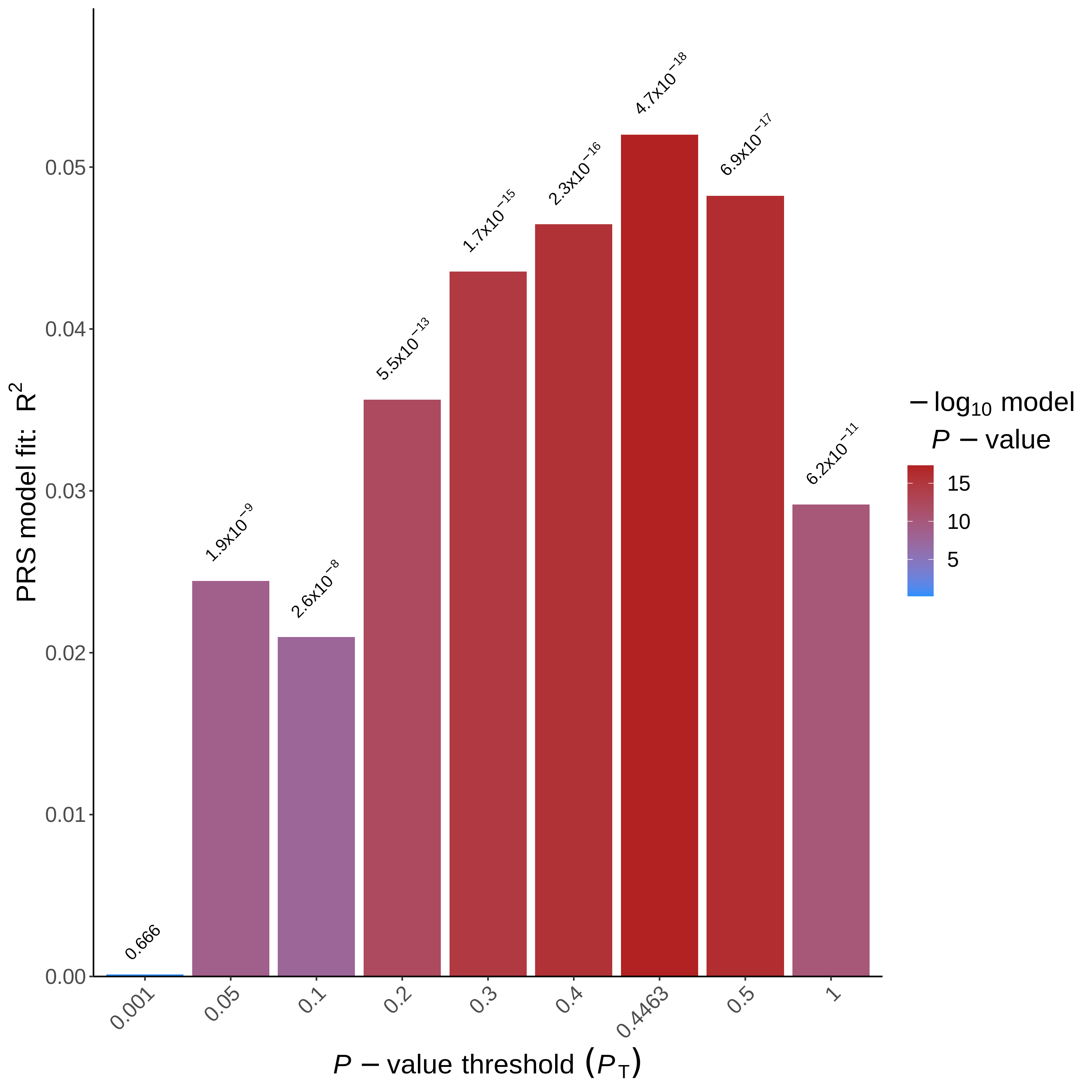
By default, PRSice saves two plots and several text files. The first plot is PRSice_BARPLOT_<date>.png(which you find in Result/GWAS6 using the file browser, the filename depends on the current date). This plot illustrates the predictive value (Nagelkerke’s R²) in the target sample based on SNPs with p-values below specific thresholds in the base sample. A p-value is also provided for each model.
Stop - Read - Solve
- Which P-value threshold generated the “best-fit” PRS?
- How much phenotypic variation does the “best-fit” PRS explain?
Hint: Check the PRSice.summary file.
Solution
As shown in the plot, a model using SNPs with a p-value < 0.4463 achieves the highest predictive value in the target sample (p-value= 4.7e-18). However, as is often the case in polygenic risk scores analysis with relatively small samples, the predictive value is relatively low (Nagelkerke’s around 5%). The text files include the exact values for each p-value threshold (check them!).
The phenotypic variation (PRS.R2) explained by these variants is 0.05.
- PRS.R2: quantifies how much of the trait variation is attributable to the genetic variants used in the analysis
- Full.R2: represents the total variance explained by the full model (genetic variants and any other covariates used)
- Null.R3: indicates the variance explained by the model without the PRS component (i.e., just the covariates)
The second plot PRSice_HIGH-RES_PLOT_<date>.png (which you again can manually open) shows many different p-value thresholds. The p-value of the predictive effect is in black together with an aggregated trend line in green.
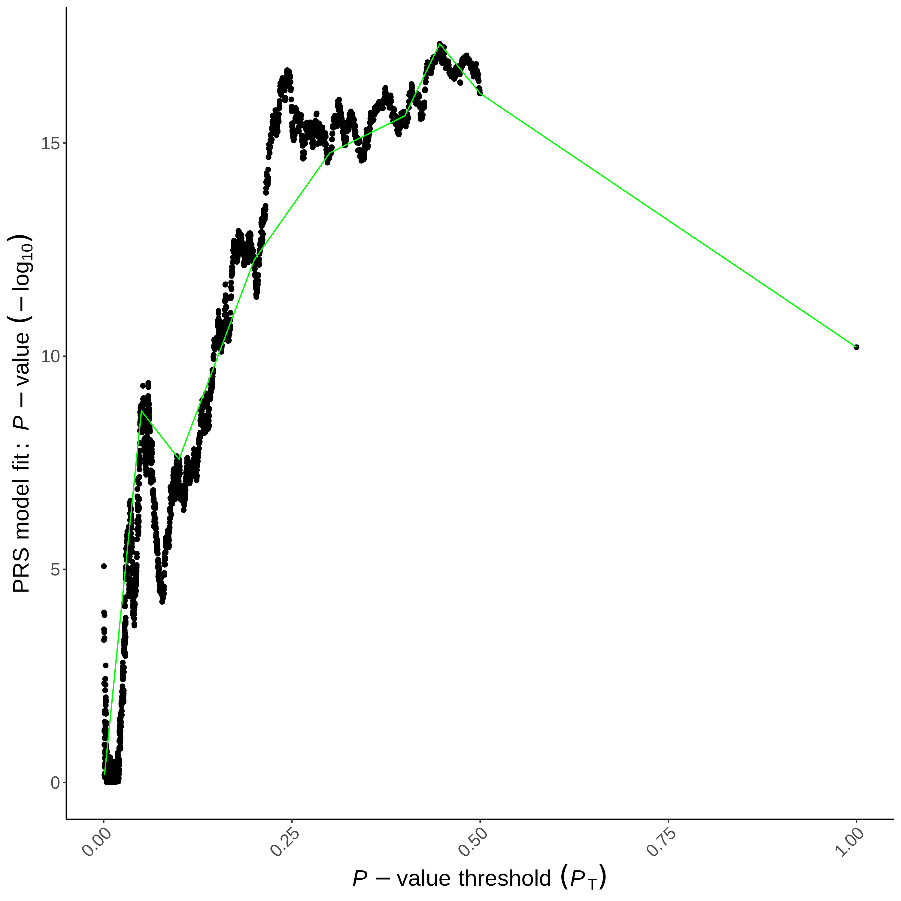
Both figures show that trait-associated SNPs in the base sample can predict the trait in the target sample. If the same trait is used, predictive power depends on the trait’s heritability and base sample size. When using related but different traits, the predictive power also depends on their genetic correlation. Studies suggest that models with more lenient p-value thresholds capture smaller effects important for complex traits, while stricter thresholds reduce noise, aiding interpretation and the understanding of the underlying genetic architecture. Balancing informative SNPs and minimizing noise is key to maximizing predictive power.
Stop - Read - Solve
- Using R, plot the scores for the “best-fit” P-value threshold against another P-value threshold of your choice.
# R code here (switch the kernel if necessary)Conclusion
In this tutorial, we have discussed how to perform a simple polygenic risk score analysis using the PRSice script and interpret its results. As mentioned before, PRSice offers many additional options to adjust the risk score analysis, including adding covariates (principal components) and adjusting clumping parameters. It is recommended to read the user manual of PRSice to perform a polygenic risk score analysis optimal to the research question at hand.
Now, you will need to do the same for a quantitative trait and explore the results.
Other take-home messages
- Replication in (several) other cohorts provides convincing evidence
- Applying stringent statistics (P<5e-8) helps to reduce the likelihood of false-positive results
- An external reference panel can be used to improve LD estimation for clumping, providing more accurate definitions of LD blocks and refining the selection of variants for PRS analysis, especially when sample size is limited (e.g. ~500 samples).
References
Berisa, Tomaz, and Joseph K Pickrell. 2016. “Approximately Independent Linkage Disequilibrium Blocks in Human Populations.” Bioinformatics 32 (2): 283.
Dudbridge, Frank. 2013. “Power and Predictive Accuracy of Polygenic Risk Scores.” PLoS Genetics 9 (3): e1003348.
Copyright
CC-BY-SA 4.0 license