Gene-level differential expression analysis with DESeq2

Approximate time: 15 minutes

Learning Objectives

• Explain the different steps involved in running DESeq()
• Examine size factors and understand the source of differences
• Inspect gene-level dispersion estimates
• Recognize the importance of dispersion during differential expression analysis

DESeq2 differential gene expression analysis workflow

Previously, we created the DESeq2 object using the appropriate design formula.

# DO NOT RUN

# Create dds object
dds <- DESeqDataSetFromTximport(txi,
                                colData = meta %>% column_to_rownames("sample"), 
                                design = ~ condition)

# Filter genes with 0 counts
keep <- rowSums(counts(dds)) > 0
dds <- dds[keep,]

Then, to run the entire differential expression analysis workflow, we use a single call to the function DESeq().

## Run analysis
dds <- DESeq(dds)

And with that we completed the entire workflow for the differential gene expression analysis with DESeq2! The DESeq() function performs a default analysis through the following steps:

1. Estimation of size factors: estimateSizeFactors()
2. Estimation of dispersion: estimateDispersions()
3. Negative Binomial GLM fitting and Wald statistics: nbinomWaldTest()

Step 1: Estimate size factors

The first step in the differential expression analysis is to estimate the size factors, which is exactly what we already did to normalize the raw counts.

Let’s take a quick look at size factor values we have for each sample:

## Check the size factors
sizeFactors(dds)

  control_3   control_2   control_1 vampirium_3 vampirium_2 vampirium_1 
  0.7501070   0.9580056   1.1134126   0.6565921   1.1418067   1.2184977 
 garlicum_3  garlicum_2 
  0.9327493   1.5527069 

These numbers should be identical to those we generated initially when we had run the function estimateSizeFactors(dds). Take a look at the total number of reads for each sample:

## Total number of raw counts per sample
colSums(counts(dds))

  control_3   control_2   control_1 vampirium_3 vampirium_2 vampirium_1 
   20257917    26156069    30817090    17054657    29573402    31589516 
 garlicum_3  garlicum_2 
   26428310    44740987 

How do the numbers correlate with the size factor?

We see that the larger size factors correspond to the samples with higher sequencing depth, which makes sense, because to generate our normalized counts we need to divide the counts by the size factors. This accounts for the differences in sequencing depth between samples.

Now take a look at the total depth after normalization using:

## Total number of normalized counts per sample
colSums(counts(dds, normalized=T))

  control_3   control_2   control_1 vampirium_3 vampirium_2 vampirium_1 
   27006701    27302628    27678052    25974507    25900533    25924969 
 garlicum_3  garlicum_2 
   28333777    28814831 

How do the values across samples compare with the total counts taken for each sample?

You might have expected the counts to be the exact same across the samples after normalization. However, DESeq2 also accounts for RNA composition during the normalization procedure. By using the median ratio value for the size factor, DESeq2 should not be biased to a large number of counts sucked up by a few DE genes; however, this may lead to the size factors being quite different than what would be anticipated just based on sequencing depth.

Step 2: Estimate gene-wise dispersion

Let’s take a look at the dispersion estimates for our Vampirium data. First, we will use the function estimateDispersions().

dds <- estimateDispersions(dds)

We can check the values using the dispersion() function and plotting it with the plotDispEsts() function:

head(dispersions(dds))

[1] 0.102415719 0.005312987 0.005241663 9.982833068 0.954109932 0.002146811

## Plot dispersion estimates
plotDispEsts(dds)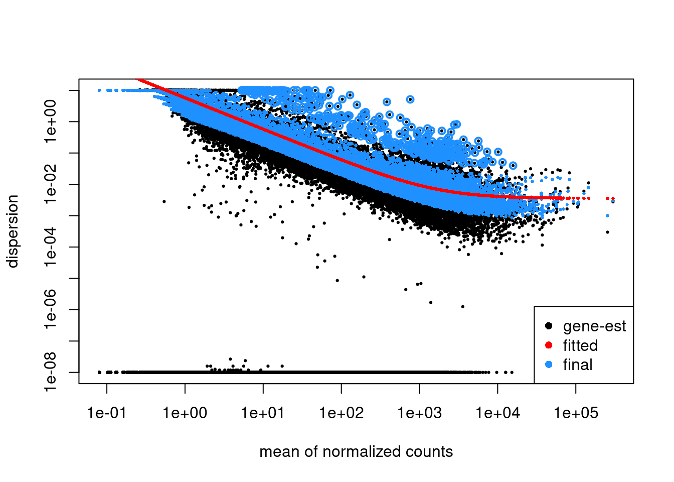

We can see that our estimated dispersions look quite good!

---

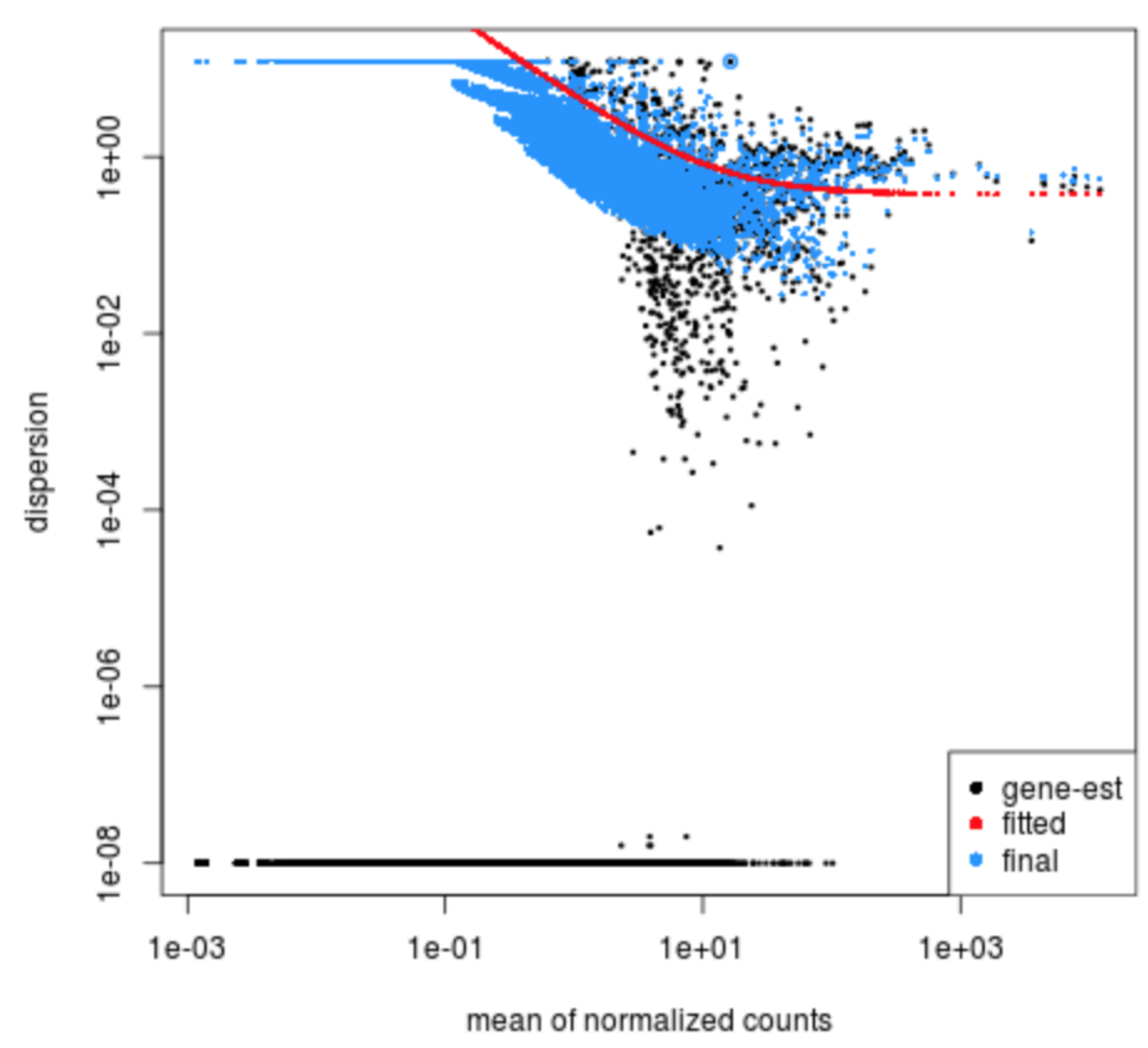
Exercise 1

Given the dispersion plot below, would you have any concerns regarding the fit of your data to the model?

• If not, what aspects of the plot makes you feel confident about your data?
• If so, what are your concerns? What would you do to address them?