library(tidyverse)
library(DESeq2)
library(ggrepel)
library(pheatmap)
library(annotables)
library(clusterProfiler)
library(DOSE)
library(pathview)
library(org.Hs.eg.db)
library(tximport)
library(RColorBrewer)Summary of DGE workflow
Approximate time: 15 minutes
Learning Objectives
- Identify the R commands needed to run a complete differential expression analysis using DESeq2
Libraries
We have detailed the various steps in a differential expression analysis workflow, providing theory with example code. To provide a more succinct reference for the code needed to run a DGE analysis, we have summarized the steps in an analysis below:
Obtaining gene-level counts from your preprocessing and create DESeq object
If you have a traditional raw count matrix
Load data and metadata
data <- read_table("../Data/Vampirium_counts_traditional.tsv")

meta <- read_csv("../Data/samplesheet.csv")
Check that the row names of the metadata equal the column names of the raw counts data
### Check that sample names match in both files
all(colnames(data)[-c(1,2)] %in% meta$sample)
[1] TRUEall(colnames(data)[-c(1,2)] == meta$sample)[1] FALSEReorder meta rows so it matches count data colnames
reorder <- match(colnames(data)[-c(1,2)],meta$sample)
reorder
[1] 3 2 1 8 7 6 5 4meta <- meta[reorder,] Create DESeq2Dataset object
dds <- DESeqDataSetFromMatrix(countData = data %>% dplyr::select(-gene_name) %>% column_to_rownames("gene_id") %>% mutate_all(as.integer),
                              colData = meta %>% column_to_rownames("sample"),
                              design = ~ condition)
If you have pseudocounts
Load samplesheet with all our metadata from our pipeline
# Load data, metadata and tx2gene and create a txi object
meta <- read_csv("../Data/samplesheet.csv")
Create a list of salmon results
dir <- "../Data/salmon"
tx2gene <- read_table(file.path(dir,"salmon_tx2gene.tsv"), col_names = c("transcript_ID","gene_ID","gene_symbol"))

# Get all salmon results files
files <- file.path(dir, meta$sample, "quant.sf")
names(files) <- meta$sample
Create txi object
txi <- tximport(files, type="salmon", tx2gene=tx2gene, countsFromAbundance = "lengthScaledTPM", ignoreTxVersion = TRUE)Create dds object
dds <- DESeqDataSetFromTximport(txi,
                                   colData = meta %>% column_to_rownames("sample"),
                              design = ~ condition)
Exploratory data analysis
Pre-filtering low count genes + PCA & hierarchical clustering - identifying outliers and sources of variation in the data:
Prefiltering low count genes
keep <- rowSums(counts(dds)) > 0
dds <- dds[keep,]
Rlog or vst transformation
# Transform counts for data visualization
rld <- rlog(dds,
            blind=TRUE)

# vsd <- vst(dds, blind = TRUE)
PCA
Plot PCA
plotPCA(rld,
        intgroup="condition")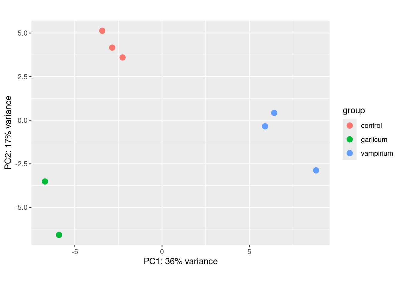
Heatmaps
Extract the rlog matrix from the object
rld_mat <- assay(rld)
rld_cor <- cor(rld_mat) # Pearson correlation between samples
rld_dist <- as.matrix(dist(t(assay(rld)))) #distances are computed by rows, so we need to transponse the matrix
Plot heatmap of correlations
pheatmap(rld_cor,
         annotation = meta %>% column_to_rownames("sample") %>% dplyr::select("condition"))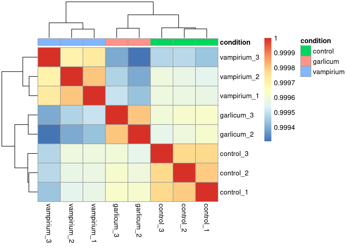
Plot heatmap of distances with a new color range
heat.colors <- brewer.pal(6, "Blues") # Colors from the RColorBrewer package (only 6)
heat.colors <- colorRampPalette(heat.colors)(100) # Interpolate 100 colors

pheatmap(rld_dist,
         annotation = meta %>% column_to_rownames("sample") %>% dplyr::select("condition"),
         color = heat.colors)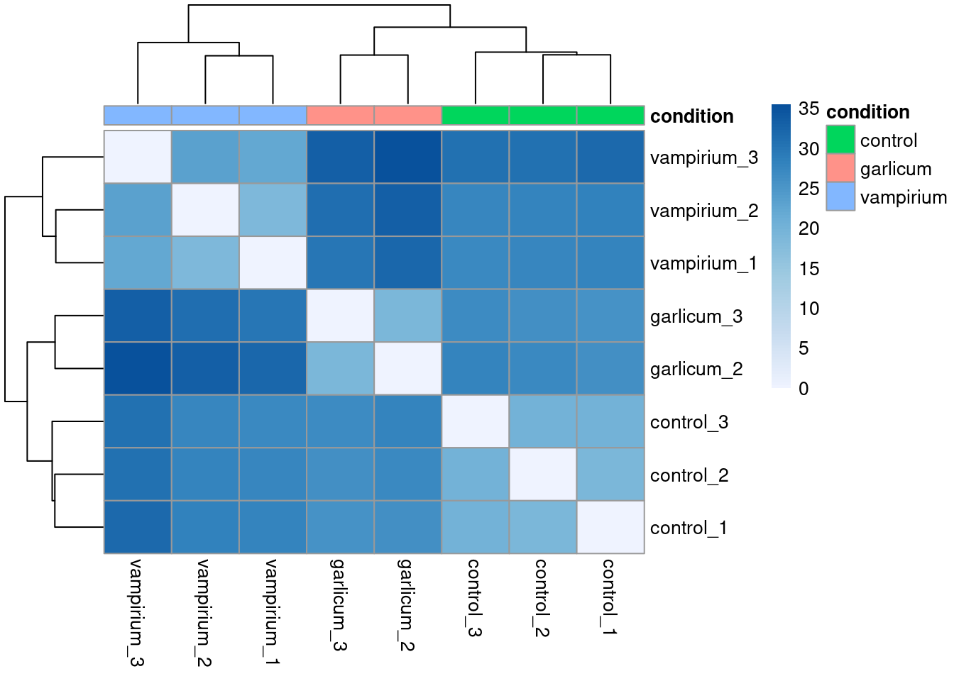
Run DESeq2:
Optional step - Re-create DESeq2 dataset if the design formula has changed after QC analysis in include other sources of variation using
# dds <- DESeqDataSetFromMatrix(data, colData = meta, design = ~ covariate + condition)Run DEseq2
# Run DESeq2 differential expression analysis
dds <- DESeq(dds)
Optional step - Output normalized counts to save as a file to access outside RStudio using
normalized_counts <- counts(dds, normalized=TRUE)Check the fit of the dispersion estimates
Plot dispersion estimates
plotDispEsts(dds)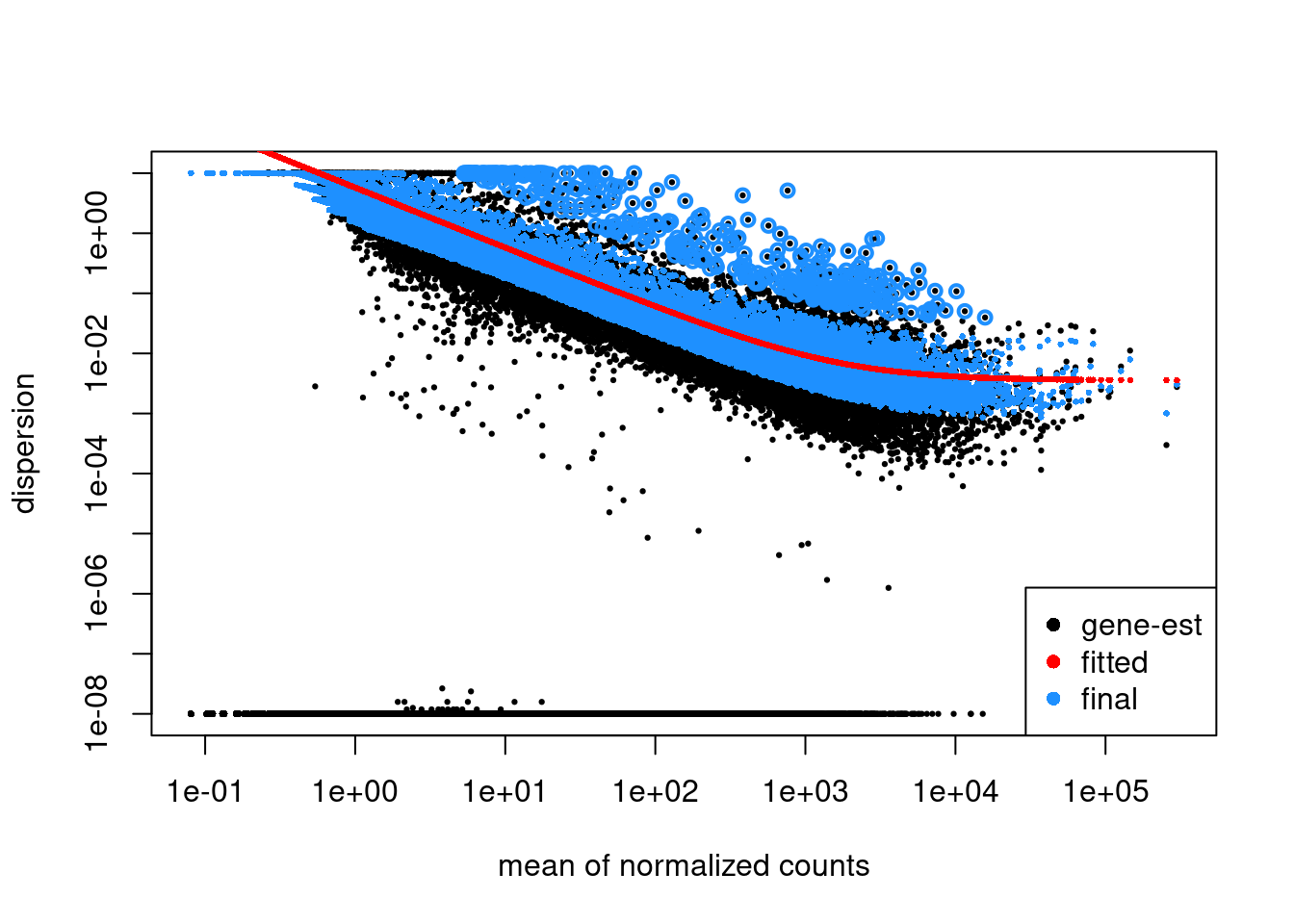
Create contrasts to perform Wald testing or the shrunken log2 fold changes between specific conditions
Formal LFC calculation
# Specify contrast for comparison of interest
contrast <- c("condition", "control", "vampirium")

# Output results of Wald test for contrast
res <- results(dds,
               contrast = contrast,
               alpha = 0.05)
Shrinkage
# Get name of the contrast you would like to use
resultsNames(dds)
[1] "Intercept" "condition_garlicum_vs_control"
[3] "condition_vampirium_vs_control"# Shrink the log2 fold changes to be more accurate
res <- lfcShrink(dds,
coef = "condition_vampirium_vs_control",
type = "apeglm")Output significant results:
# Set thresholds
padj.cutoff <- 0.05

# Turn the results object into a tibble for use with tidyverse functions
res_tbl <- res %>%
  data.frame() %>%
  rownames_to_column(var="gene") %>%
  as_tibble()

# Subset the significant results
sig_res <- dplyr::filter(res_tbl,
                  padj < padj.cutoff)
Visualize results: volcano plots, heatmaps, normalized counts plots of top genes, etc.
Function to get gene_IDs based on gene names. The function will take as input a vector of gene names of interest, the tx2gene dataframe and the dds object that you analyzed.
lookup <- function(gene_name, tx2gene, dds){
  hits <- tx2gene %>% dplyr::select(gene_symbol, gene_ID) %>% distinct() %>%
    dplyr::filter(gene_symbol %in% gene_name & gene_ID %in% rownames(dds))
  return(hits)
}

lookup(gene_name = "TSPAN7", tx2gene = tx2gene, dds = dds)
Plot expression for single gene
plotCounts(dds, gene="ENSG00000156298", intgroup="condition")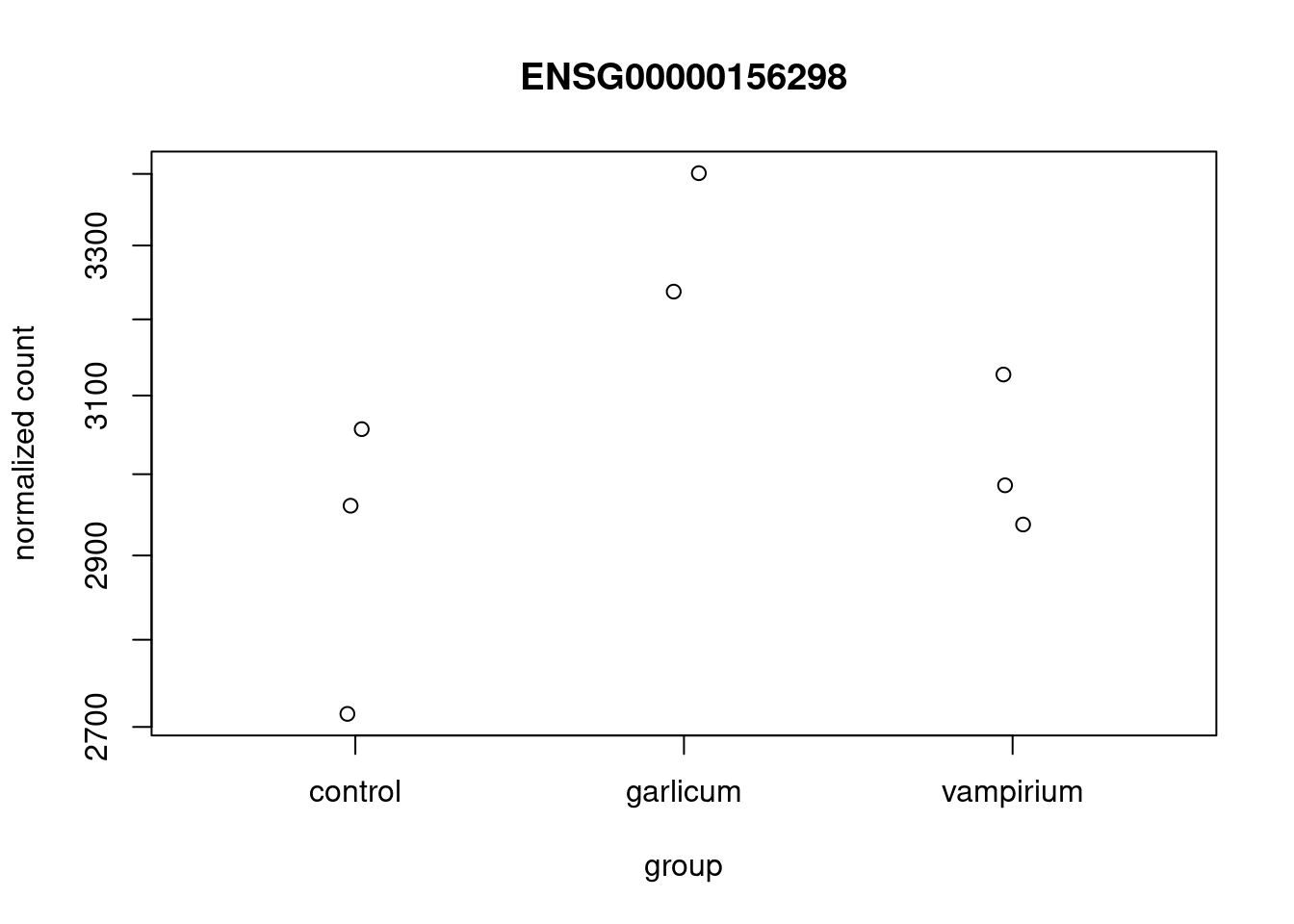
Function to annotate all your gene results
res_tbl <- merge(res_tbl, tx2gene %>% dplyr::select(-transcript_ID) %>% distinct(),
                        by.x = "gene", by.y = "gene_ID", all.x = T)

res_tbl
MAplot
plotMA(res)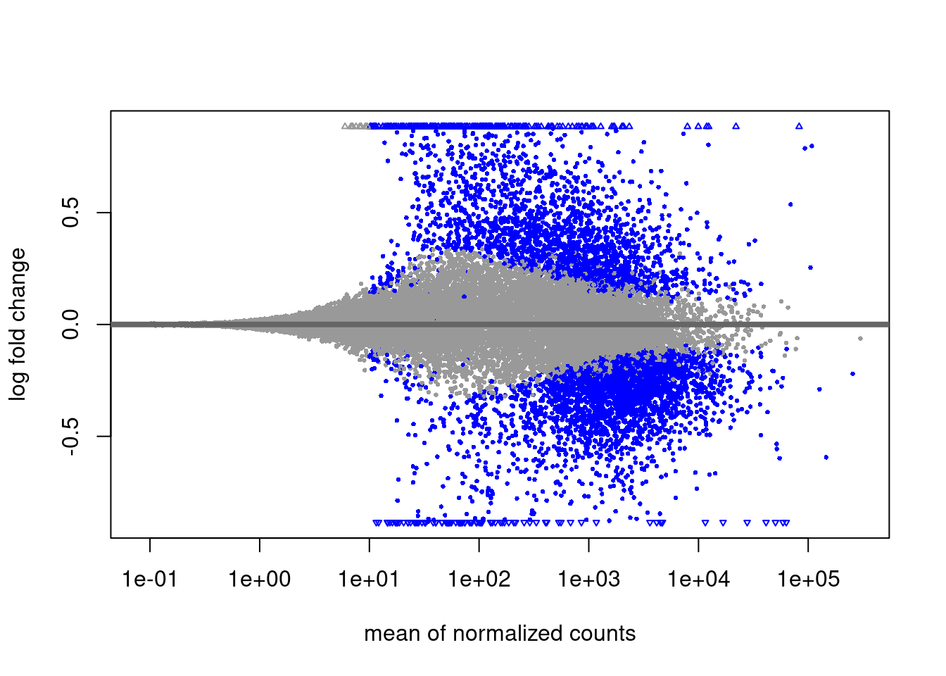
Volcano plot with labels (top N genes)
## Obtain logical vector where TRUE values denote padj values < 0.05 and fold change > 1.5 in either direction
res_tbl <- res_tbl %>%
mutate(threshold = padj < 0.05 & abs(log2FoldChange) >= 0.58)
## Create an empty column to indicate which genes to label
res_tbl <- res_tbl %>% mutate(genelabels = "")
## Sort by padj values
res_tbl <- res_tbl %>% arrange(padj)
## Populate the genelabels column with contents of the gene symbols column for the first 10 rows, i.e. the top 10 most significantly expressed genes
res_tbl$genelabels[1:10] <- as.character(res_tbl$gene[1:10])
head(res_tbl)ggplot(res_tbl, aes(x = log2FoldChange, y = -log10(padj))) +
geom_point(aes(colour = threshold)) +
geom_text_repel(aes(label = genelabels)) +
ggtitle("Vampirium vs Control") +
xlab("log2 fold change") +
ylab("-log10 adjusted p-value") +
theme(legend.position = "none",
plot.title = element_text(size = rel(1.5), hjust = 0.5),
axis.title = element_text(size = rel(1.25))) 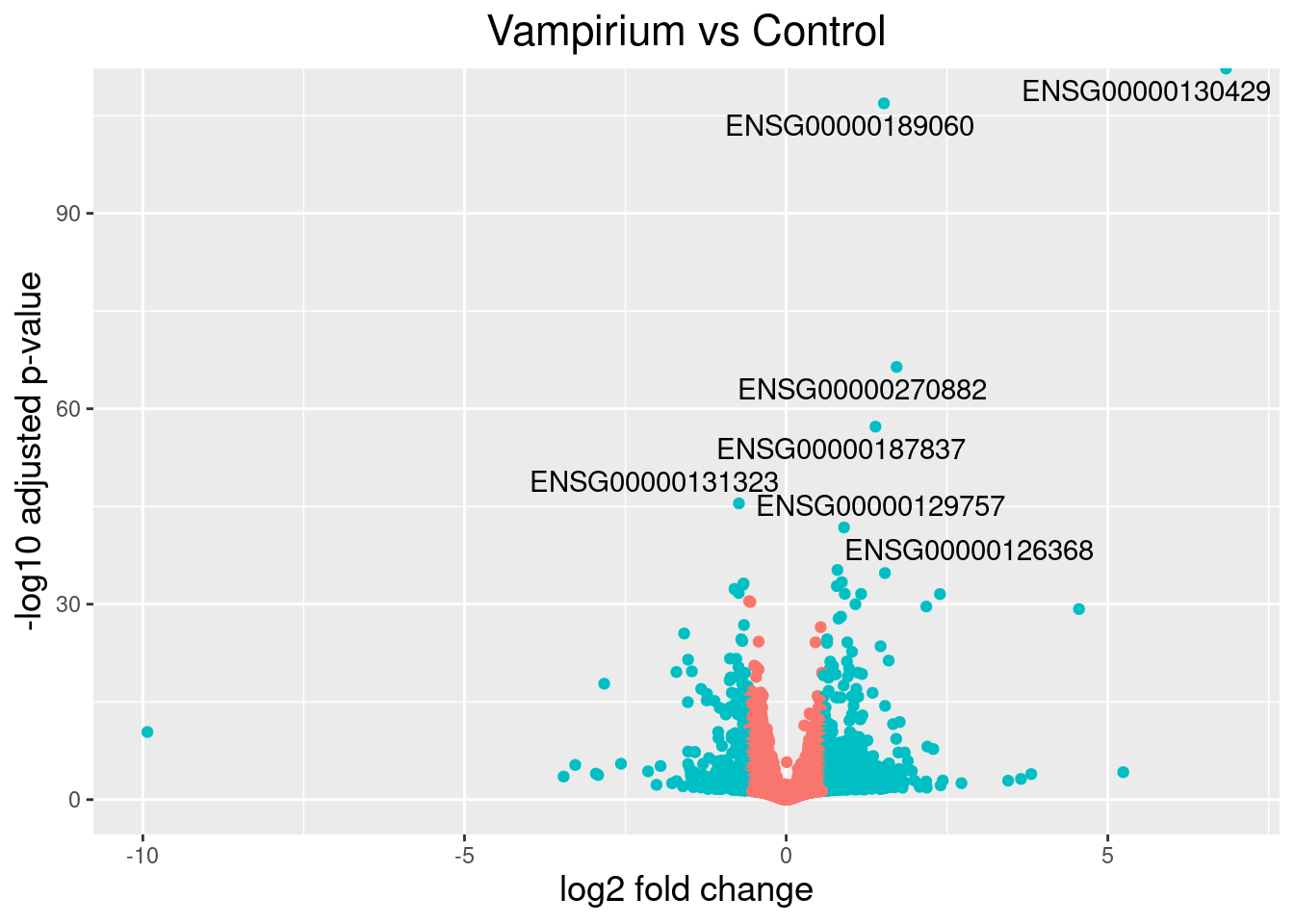
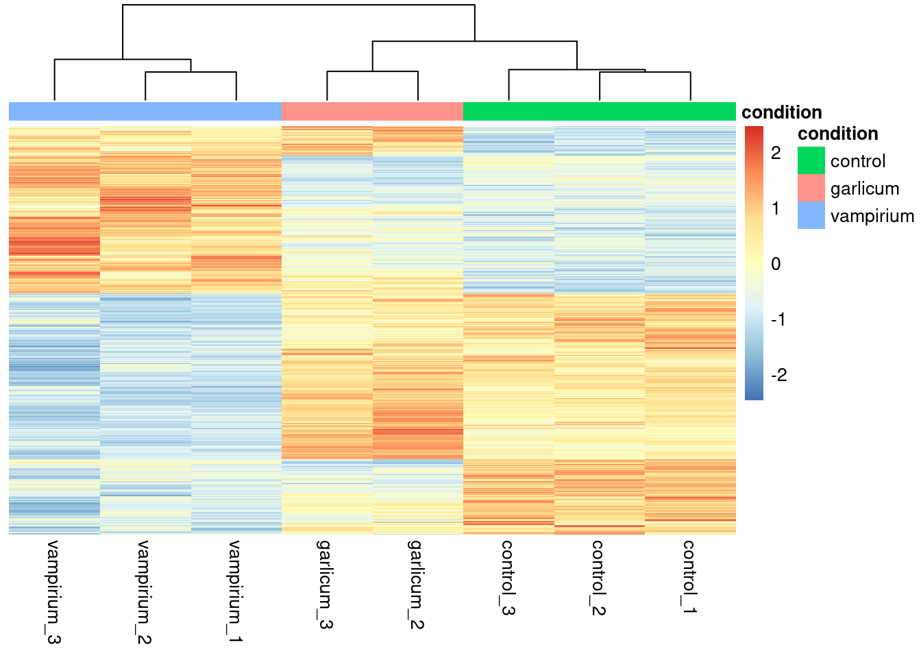
Heatmap of differentially expressed genes
# filter significant results from normalized counts
norm_sig <- normalized_counts %>% as_tibble(rownames = "gene") %>%
dplyr::filter(gene %in% sig_res$gene) %>% column_to_rownames(var="gene")pheatmap(norm_sig,
cluster_rows = T, #cluster by expression pattern
scale = "row", # scale by gene so expression pattern is visible
treeheight_row = 0, # dont show the row dendogram
show_rownames = F, # remove rownames so it is more clear
annotation = meta %>% column_to_rownames(var = "sample") %>% dplyr::select("condition")
)
Perform analysis to extract functional significance of results: GO or KEGG enrichment, GSEA, etc.
Annotate with annotables
ids <- grch38 %>% dplyr::filter(ensgene %in% res_tbl$gene)
res_ids <- inner_join(res_tbl, ids, by=c("gene"="ensgene"))
Perform enrichment analysis of GO terms (can be done as well with KEGG pathways)
# Create background dataset for hypergeometric testing using all genes tested for significance in the results
all_genes <- dplyr::filter(res_ids, !is.na(gene)) %>%
  pull(gene) %>%
  as.character()

# Extract significant results
sig <- dplyr::filter(res_ids, padj < 0.05 & !is.na(gene))

sig_genes <- sig %>%
  pull(gene) %>%
  as.character()
# Perform enrichment analysis
ego <- enrichGO(gene = sig_genes,
universe = all_genes,
keyType = "ENSEMBL",
OrgDb = org.Hs.eg.db,
ont = "BP",
pAdjustMethod = "BH",
qvalueCutoff = 0.05,
readable = TRUE)
ego <- enrichplot::pairwise_termsim(ego)Visualize result
dotplot(ego, showCategory=50)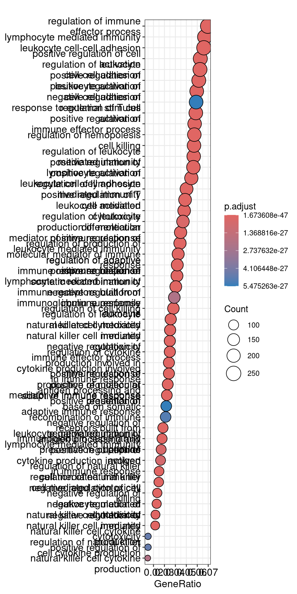
emapplot(ego, showCategory = 50)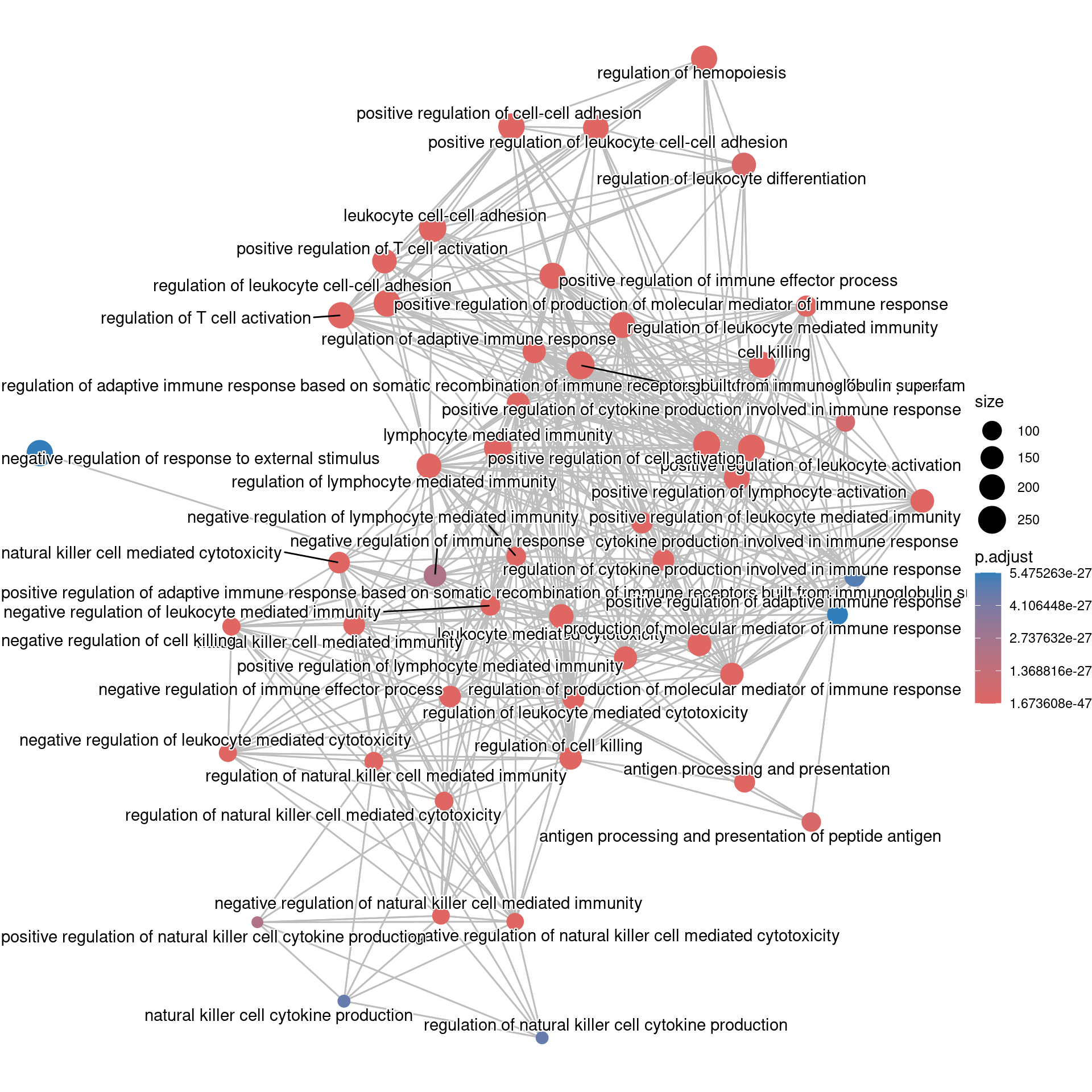
Cnetplot
## To color genes by log2 fold changes, we need to extract the log2 fold changes from our results table creating a named vector
sig_foldchanges <- sig$log2FoldChange

names(sig_foldchanges) <- sig$gene
## Cnetplot details the genes associated with one or more terms - by default gives the top 5 significant terms (by padj)
cnetplot(ego,
categorySize="pvalue",
showCategory = 5,
foldChange=sig_foldchanges,
vertex.label.font=6)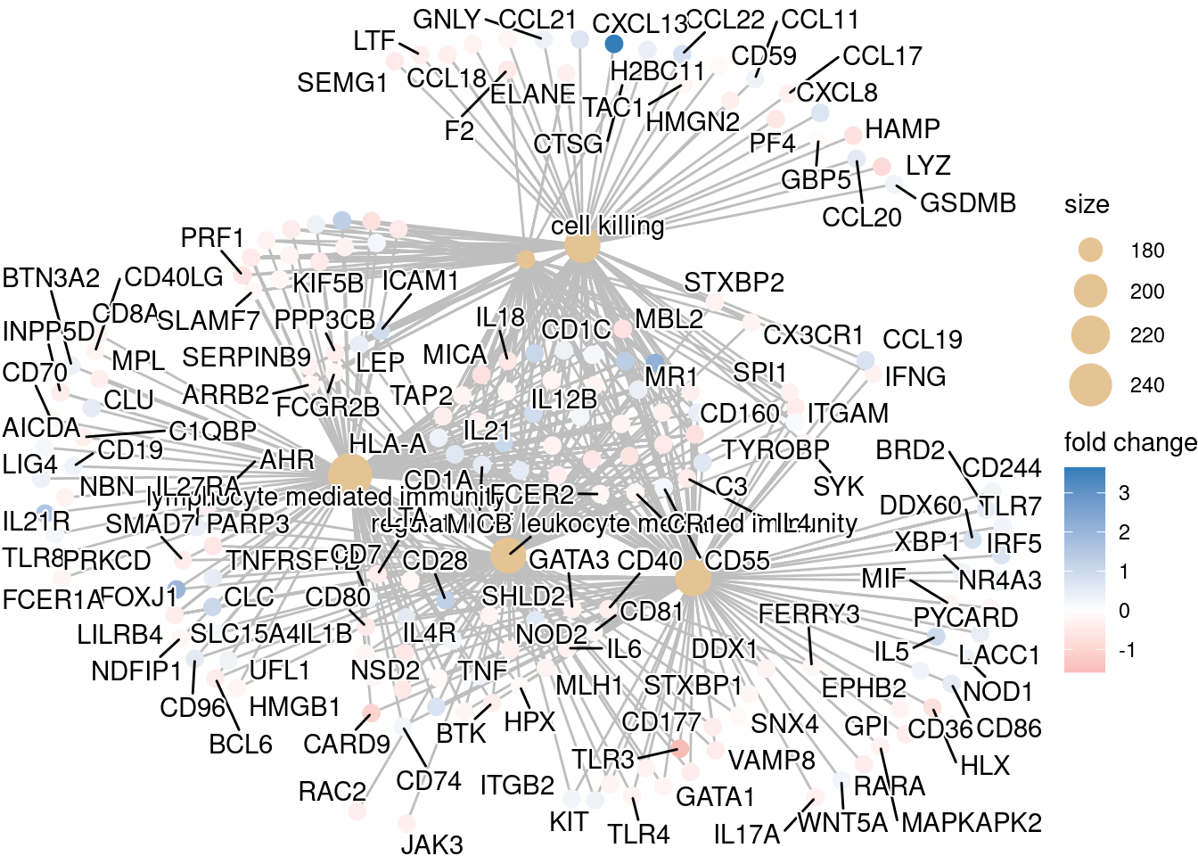
Perform GSEA analysis of KEGG pathways (can be done as well with GO terms)
# Extract entrez IDs. IDs should not be duplicated or NA
res_entrez <- dplyr::filter(res_ids, entrez != "NA" & entrez != "NULL" & duplicated(entrez)==F)

## Extract the foldchanges
foldchanges <- res_entrez$log2FoldChange

## Name each fold change with the corresponding Entrez ID
names(foldchanges) <- res_entrez$entrez

## Sort fold changes in decreasing order
foldchanges <- sort(foldchanges, decreasing = TRUE)
# Run GSEA of KEGG
gseaKEGG <- gseKEGG(geneList = foldchanges, # ordered named vector of fold changes (Entrez IDs are the associated names)
organism = "hsa", # supported organisms listed below
pvalueCutoff = 0.05, # padj cutoff value
verbose = FALSE)
gseaKEGG_results <- gseaKEGG@result
head(gseaKEGG_results)## Plot the GSEA plot for a single enriched pathway:
gseaplot(gseaKEGG, geneSetID = gseaKEGG_results$ID[1])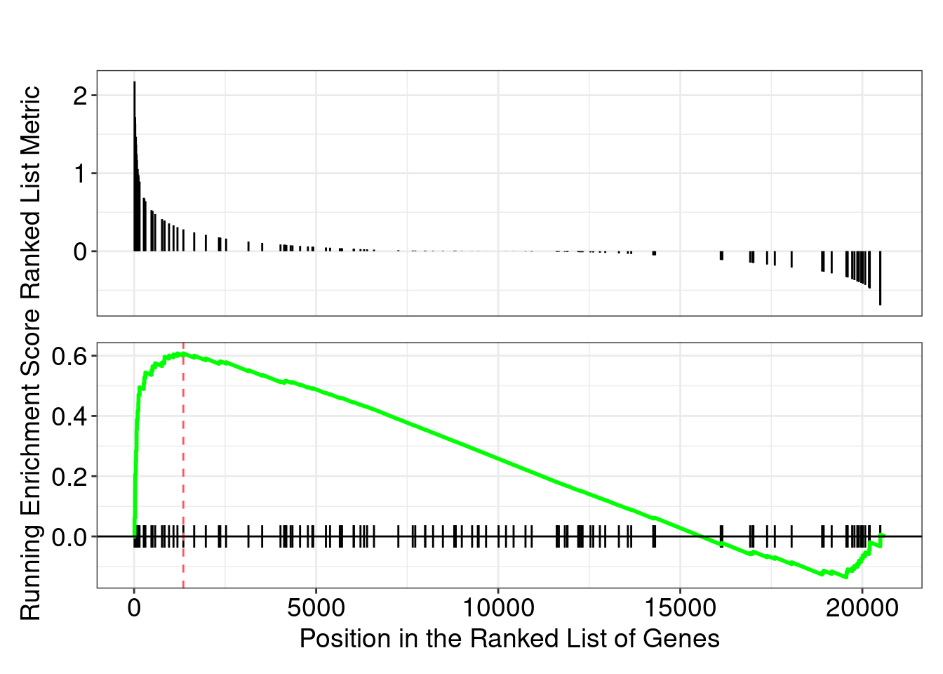
## Output images for a single significant KEGG pathway
pathview(gene.data = foldchanges,
              pathway.id = gseaKEGG_results$ID[1],
              species = "hsa",
              limit = list(gene = 2, # value gives the max/min limit for foldchanges
cpd = 1))knitr::include_graphics(paste0("./",gseaKEGG_results$ID[1],".png"))
Make sure to output the versions of all tools used in the DE analysis:
sessionInfo()R version 4.4.2 (2024-10-31)
Platform: x86_64-pc-linux-gnu
Running under: Ubuntu 24.04.1 LTS
Matrix products: default
BLAS: /usr/lib/x86_64-linux-gnu/openblas-pthread/libblas.so.3
LAPACK: /usr/lib/x86_64-linux-gnu/openblas-pthread/libopenblasp-r0.3.26.so; LAPACK version 3.12.0
locale:
[1] LC_CTYPE=C.UTF-8 LC_NUMERIC=C LC_TIME=C.UTF-8
[4] LC_COLLATE=C.UTF-8 LC_MONETARY=C.UTF-8 LC_MESSAGES=C.UTF-8
[7] LC_PAPER=C.UTF-8 LC_NAME=C LC_ADDRESS=C
[10] LC_TELEPHONE=C LC_MEASUREMENT=C.UTF-8 LC_IDENTIFICATION=C
time zone: UTC
tzcode source: system (glibc)
attached base packages:
[1] stats4 stats graphics grDevices datasets utils methods
[8] base
other attached packages:
[1] RColorBrewer_1.1-3 tximport_1.34.0
[3] org.Hs.eg.db_3.20.0 AnnotationDbi_1.68.0
[5] pathview_1.46.0 DOSE_4.0.0
[7] clusterProfiler_4.14.4 annotables_0.2.0
[9] pheatmap_1.0.12 ggrepel_0.9.6
[11] DESeq2_1.46.0 SummarizedExperiment_1.36.0
[13] Biobase_2.66.0 MatrixGenerics_1.18.1
[15] matrixStats_1.5.0 GenomicRanges_1.58.0
[17] GenomeInfoDb_1.42.1 IRanges_2.40.1
[19] S4Vectors_0.44.0 BiocGenerics_0.52.0
[21] lubridate_1.9.4 forcats_1.0.0
[23] stringr_1.5.1 dplyr_1.1.4
[25] purrr_1.0.2 readr_2.1.5
[27] tidyr_1.3.1 tibble_3.2.1
[29] ggplot2_3.5.1 tidyverse_2.0.0
loaded via a namespace (and not attached):
[1] jsonlite_1.8.9 magrittr_2.0.3 ggtangle_0.0.6
[4] farver_2.1.2 rmarkdown_2.29 fs_1.6.5
[7] zlibbioc_1.52.0 vctrs_0.6.5 memoise_2.0.1
[10] RCurl_1.98-1.16 ggtree_3.14.0 htmltools_0.5.8.1
[13] S4Arrays_1.6.0 SparseArray_1.6.1 gridGraphics_0.5-1
[16] htmlwidgets_1.6.4 plyr_1.8.9 cachem_1.1.0
[19] igraph_2.1.4 lifecycle_1.0.4 pkgconfig_2.0.3
[22] Matrix_1.7-1 R6_2.5.1 fastmap_1.2.0
[25] gson_0.1.0 GenomeInfoDbData_1.2.13 numDeriv_2016.8-1.1
[28] digest_0.6.37 aplot_0.2.4 enrichplot_1.26.6
[31] colorspace_2.1-1 patchwork_1.3.0 RSQLite_2.3.9
[34] labeling_0.4.3 timechange_0.3.0 httr_1.4.7
[37] abind_1.4-8 compiler_4.4.2 bit64_4.6.0-1
[40] withr_3.0.2 BiocParallel_1.36.0 DBI_1.2.3
[43] R.utils_2.12.3 MASS_7.3-61 DelayedArray_0.32.0
[46] tools_4.4.2 ape_5.8-1 R.oo_1.27.0
[49] glue_1.8.0 nlme_3.1-166 GOSemSim_2.32.0
[52] grid_4.4.2 reshape2_1.4.4 fgsea_1.33.1
[55] generics_0.1.3 gtable_0.3.6 tzdb_0.4.0
[58] R.methodsS3_1.8.2 data.table_1.16.4 hms_1.1.3
[61] XVector_0.46.0 pillar_1.10.1 emdbook_1.3.13
[64] vroom_1.6.5 yulab.utils_0.1.9 splines_4.4.2
[67] treeio_1.30.0 lattice_0.22-6 renv_1.0.11
[70] bit_4.5.0.1 tidyselect_1.2.1 GO.db_3.20.0
[73] locfit_1.5-9.10 Biostrings_2.74.1 knitr_1.49
[76] xfun_0.50 KEGGgraph_1.66.0 stringi_1.8.4
[79] UCSC.utils_1.2.0 lazyeval_0.2.2 ggfun_0.1.8
[82] yaml_2.3.10 evaluate_1.0.3 codetools_0.2-20
[85] bbmle_1.0.25.1 qvalue_2.38.0 Rgraphviz_2.50.0
[88] BiocManager_1.30.25 graph_1.84.1 ggplotify_0.1.2
[91] cli_3.6.3 munsell_0.5.1 Rcpp_1.0.14
[94] coda_0.19-4.1 png_0.1-8 bdsmatrix_1.3-7
[97] XML_3.99-0.18 parallel_4.4.2 blob_1.2.4
[100] bitops_1.0-9 mvtnorm_1.3-3 apeglm_1.28.0
[103] tidytree_0.4.6 scales_1.3.0 crayon_1.5.3
[106] rlang_1.1.5 cowplot_1.1.3 fastmatch_1.1-6
[109] KEGGREST_1.46.0